OVERVIEW
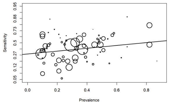
By its nature of combining studies to summarize the effectiveness of an index test compared with a reference test, meta-analyses are prone to between-study variability. There are many ways to investigate and explain such heterogeneity in terms of study-level variables. One of them is to perform meta-regression.
In this blog , we go over each step of a program in the R language (Team (2020)) designed to investigate heterogeneity by comparing summary points. The program uses the rjags package (an interface to the JAGS library (Plummer (2003)) in order to draw samples from the posterior distribution of the parameters using Markov Chain Monte Carlo (MCMC) methods. It relies on the mcmcplots package to assess convergence of the meta-analysis model. It returns summary statistics on the mean sensitivity and specificity across studies and between-study heterogeneity. A summary plot in ROC space can be created with the help of the DTAplots package.
MOTIVATING EXAMPLE AND DATA
We illustrate the script by applying it to a data from a systematic review of studies evaluating the accuracy of two different generations of the Anti-cyclic citrullinated peptide (Anti-CCP) test for rheumatoid arthritis (index test) compared to the 1987 revised American college or Rheumatology (ACR) criteria or clinical diagnosis (reference test) for 37 studies (Nishimura et al. (2007)). In this example, it is assume that the diagnostic accuracy of Anti-CCP test may vary according to the different CCP generation. Each study provides a two-by-two table of the form
| Disease_positive | Disease_negative | |
|---|---|---|
| Inex test positive | TP | FP |
| Index test negative | FN | TN |
where:
TPis the number of individuals who tested positive on both testsFPis the number of individuals who tested positive on the index test and negative on the reference testFNis the number of individuals who tested negative on the index test and positive on the reference testTNis the number of individuals who tested negative on both tests
The studies included in the review to assess the diagnostic performance of anti-CCP used two different generations of the assay: first generation (CCP1) had 8 studies and second generation (CCP2) had 29 studies. Each study can be related to its CCP generation through a dichotomous covariate of the form
\[ \begin{equation} Z_i= \begin{cases} 1 & \text{if CCP second generation (CCP2)} \\ 0 & \text{if CCP first generation (CCP1)} \end{cases}\end{equation} \]
TP=c(115, 110, 40, 23, 236, 74, 89, 90, 31, 69, 25, 43, 70, 167, 26, 110, 26, 64, 71, 68, 38, 42, 149, 147, 47, 24, 40, 171, 72, 7, 481, 190, 82, 865, 139, 69, 90)

FP=c(17, 24, 5, 0, 20, 11, 4, 2, 0, 8, 2, 1, 5, 8, 8, 3, 1, 14, 2, 14, 3, 2, 7, 10, 7, 3, 11, 26, 14, 2, 23, 12, 13, 79, 7, 5, 7)

FN=c(16, 86, 58, 7, 88, 8, 29, 50, 22, 18, 10, 63, 17, 98, 15, 148, 20, 15, 58, 35, 0, 60, 109, 35, 20, 18, 46, 60, 77, 9, 68, 105, 71, 252, 101, 107, 101)

TN=c(73, 215, 227, 39, 231, 130, 142, 129, 75, 38, 40, 120, 228, 88, 15, 118, 56, 293, 66, 132, 73, 96, 114, 106, 375, 79, 146, 443, 298, 51, 185, 408, 301, 2218, 464, 133, 313)

Z=c(1,0,0,1,1,1,1,1,1,1,1,0,1,1,1,0,1,1,1,1,1,1,1,1,1,1,0,1,0,1,1,1,1,1,0,1,0)

pos= TP + FN
neg= TN + FP
n <- length(TP) #  Number of studies
dataList = list(TP=TP,TN=TN,n=n,pos=pos,neg=neg, Z=Z)
THE MODEL
The meta-regression model is an extension of the hierarchical meta-analysis model we have already discussed in this blog. Under the assumption of equal variances of the random effects for the logit sensitivities and the logit specificities, we have
- Within-study level: In each study, TP is assumed to follow a Binomial distribution with probability equal to the sensitivity and TN is assumed to follow a Binomial distribution with probability equal to the specificity.
- Between-study level: The logit transformed sensitivity (\(\mu_{1i}\)) and the logit transformed specificity (\(\mu_{2i}\)) in each study jointly follow a bivariate normal distribution:
\[ \begin{pmatrix} \mu_{1i} \\ \mu_{2i} \\ \end{pmatrix} \sim N \begin{pmatrix} \begin{pmatrix} \mu_{1} + \nu_{1}Z_i \\ \mu_{2} + \nu_{2}Z_i \\ \end{pmatrix}, \Sigma_{12} \end{pmatrix} \text{with } \Sigma\_{12} = \begin{pmatrix} \tau_{1}^2 & \rho \tau_1 \tau_2\\ \rho \tau_1 \tau_2 & \tau_2^2 \\ \end{pmatrix} \]
where \(\nu_1\) and \(\nu_2\) are the logit mean difference between CCP2 and CCP1 in sensitivity and specificity, respectively, \(\tau_1^2\) and \(\tau_2^2\) are the between-study variance parameters and \(\rho\) is the correlation between \(\mu_{1i}\) and \(\mu_{2i}\).
The model is written in JAGS syntax, and stored in a character object that we called modelString which is later saved in the current working directory via the R function writeLines.
Any parameters that are function of the parameters defined in the likelihood above can easily be derived in a Bayesian framework by adding a coupe of lines to the JAGS model. In the PARAMETERS OF INTEREST section of the JAGS model below, we derive a few extra parameters we might be interested in. For instance, this is where the parameters Difference_Se and Difference_Sp monitoring the diagnostic accuracy comparison between the 2 CCP generations are derived. We arbitrarily made that difference such that it will be positive if the accuracy of CCP2 is greater than CCP1 and negative if the accuracy of CCP2 is less than CCP1.
Using JAGS built in step function we are able to also define parameters that estimate the posterior probability that the accuracy of CCP2 is greater than CCP1 (Prob_Se and Prob_Sp). The step function evaluate a certain condition and results in a 0-1 dichotomous response whether the condition was met or not. For example,Prob_Se is defined below to evaluate at each iteration sampling step if the summary sensitivity estimate of CCP2 is greater than the summary sensitivity of CCP1. When it is, Prob_Se is assigned a value of 1 by the step function. When it’s not, Prob_Se is set to 0. Upon completion of the MCMC sampling process, Prob_Se is therefore the posterior probability that the summary sensitivity of CCP2 is greater than summary sensitivity of CCP1, with the following interpretation :
- A posterior probability
Prob_Seequals to 0.5 would mean that the sensitivity of both CCP2 and CCP1 are equal - A posterior probability
Prob_Segreater than 0.5 would mean that the sensitivity of CCP2 tend to be greater than CCP1.
- A posterior probability
Prob_Seless than 0.5 would mean that the sensitivity of CCP2 tend to be lower than CCP1.
modelString =

  "model {
#=== LIKELIHOOD ===#
for(i in 1:n) {
TP[i] ~ dbin(se[i],pos[i])
TN[i] ~ dbin(sp[i],neg[i])
# === PRIOR FOR INDIVIDUAL LOGIT SENSITIVITY AND SPECIFICITY === #
logit(se[i]) <- l[i,1]
logit(sp[i]) <- l[i,2]
mu_reg[i,1] <- mu[1] + nu[1]*Z[i]
mu_reg[i,2] <- mu[2] + nu[2]*Z[i]
l[i,1:2] ~ dmnorm(mu_reg[i,], T[,])
}
#=== HYPER PRIOR DISTRIBUTIONS MEAN LOGIT SENSITIVITY AND SPECIFICITY === #
mu[1] ~ dnorm(0,0.3)
mu[2] ~ dnorm(0,0.3)
nu[1] ~ dnorm(0, 0.3)
nu[2] ~ dnorm(0, 0.3)

# Between-study variance-covariance matrix (TAU)
T[1:2,1:2]<-inverse(TAU[1:2,1:2])
TAU[1,1] <- tau[1]*tau[1]
TAU[2,2] <- tau[2]*tau[2]
TAU[1,2] <- rho*tau[1]*tau[2]
TAU[2,1] <- rho*tau[1]*tau[2]

#=== HYPER PRIOR DISTRIBUTIONS FOR PRECISION OF LOGIT SENSITIVITY ===#
#=== AND LOGIT SPECIFICITY, AND CORRELATION BETWEEN THEM === #
prec[1] ~ dgamma(2,0.5)
prec[2] ~ dgamma(2,0.5)
rho ~ dunif(-1,1)

# ===  PARAMETERS OF INTEREST === #

# BETWEEN-STUDY VARIANCE (tau.sq) AND STANDARD DEVIATION (tau) OF LOGIT SENSITIVITY AND SPECIFICITY
tau.sq[1]<-pow(prec[1],-1)
tau.sq[2]<-pow(prec[2],-1)
tau[1]<-pow(prec[1],-0.5)
tau[2]<-pow(prec[2],-0.5)

# SUMMARY SENSITIVITY AND SPECIFICITY OF CCP1
Summary_Se_CCP1<-1/(1+exp(-mu[1]))
Summary_Sp_CCP1<-1/(1+exp(-mu[2]))
# SUMMARY SENSITIVITY AND SPECIFICITY OF CCP2
Summary_Se_CCP2<-1/(1+exp(-mu[1] - nu[1]))
Summary_Sp_CCP2<-1/(1+exp(-mu[2] - nu[2]))
# PREDICTED SENSITIVITY AND SPECIFICITY IN A NEW STUDY EVALUATING CCP1
l_CCP1_new[1:2] ~ dmnorm(mu[],T[,])
Predicted_Se_CCP1 <- 1/(1+exp(-l_CCP1_new[1]))
Predicted_Sp_CCP1 <- 1/(1+exp(-l_CCP1_new[2]))
# PREDICTED SENSITIVITY AND SPECIFICITY IN A NEW STUDY EVALUATING CCP2
mu_new[1] <- mu[1] + nu[1]
mu_new[2] <- mu[2] + nu[2]
l_CCP2_new[1:2] ~ dmnorm(mu_new[],T[,])
Predicted_Se_CCP2 <- 1/(1+exp(-l_CCP2_new[1]))
Predicted_Sp_CCP2 <- 1/(1+exp(-l_CCP2_new[2]))

# POSTERIOR DIFFERENCES\ PROBABILITIES
Difference_Se <- Summary_Se_CCP2 - Summary_Se_CCP1
Difference_Sp <- Summary_Sp_CCP2 - Summary_Sp_CCP1

Prob_Se <- step(Difference_Se)
Prob_Sp <- step(Difference_Sp)
}
"

writeLines(modelString,con="model.txt")
INTIAL VALUES
Running multiple chains, each starting at different initial values, serves to assess convergence of the MCMC algorithm by examining if all chains reach the same solution. In JAGS, initial values must be stored in a list object, one list for each chain. So when running multiple chains, initial values should be provided as a list of lists. In the illustration below we give details on how to provide initial values chosen by the user by using a homemade function we are calling GenInits().
Providing relevant initial values can speed up convergence of the MCMC algorithm. Here we create a function that allows us to provide our own initial values for the logit-transformed sensitivity (mu[1]) and logit-transformed specificity (mu[2]) parameters. We can provide specific initial values to mu[1] and mu[2] through the init_mu argument or we can use the function to randomly generate initial values from a normal distribution (corresponding to the prior distribution found in the model) for mu[1] and mu[2]. In this example, we have allowed other parameters, such as logit mean difference between CCP2 and CCP1 in sensitivity and specificity (nu[1] and nu[2]), between-study precisions (prec[1] and prec[2]) and correlation between logit-transformed sensitivity and logit-transformed specificity (rho) to be randomly generated according to their prior distribution by GenInits(). In our experience, choosing initial values for these parameters is not easy. For reproducibility, a Seed argument is provided.
In the illustration below, we set mu[1] and mu[2] equal to 0 (which represents an initial value of 0.5 on the probability scale) for the first chain. For chains number 2 and 3, we simply set the argument init_mu to NULL. This ensures both chain 2 and chain 3 are randomly initialized.
# Initial values
GenInits = function(init_mu=NULL, Seed){
  if(is.null(init_mu) == "FALSE"){
    mu = c(as.numeric(init_mu[1]),as.numeric(init_mu[2]))
  }
  else{
    mu=c(rnorm(1,0,1/sqrt(0.3)),rnorm(1,0,1/sqrt(0.3)))
  }
  list(
    mu=mu,
    nu=c(rnorm(1,0,1/sqrt(0.3)),rnorm(1,0,1/sqrt(0.3))),
    prec = c(rgamma(1,2,0.5),rgamma(1,2,0.5)),
    rho = runif(1,-1,1),
    .RNG.name="base::Wichmann-Hill",
    .RNG.seed=Seed
  )
}
seed=123
set.seed(seed)
Listinits = list(
  GenInits(init_mu=c(0,0), Seed=seed),
  GenInits(Seed=seed),
  GenInits(Seed=seed)
)
COMPILING AND RUNNING THE MODEL
The jags.model function compiles the model for possible syntax errors. Argument n.chains=3 creates 3 MCMC chains with different starting values given by the Listinits object defined above.
library(rjags)
# Compile the model
jagsModel = jags.model("model.txt",data=dataList,n.chains=3,inits=Listinits)
The update function serves as to carry out the “burn-in” step. This corresponds to discarding initial iterations till the MCMC algorithm has reached its equilibrium distribution. Here we chose to discard 30,000 iterations by providing argument n.iter=30000. This can be helpful to mitigate “bad” initial values.
# Burn-in iterations
update(jagsModel,n.iter=30000)
The coda.samples function draws samples from the posterior distribution of the unknown parameters that were defined in the parameters object. Here we are drawing n.iter=30000 iterations from the posterior distributions for each chain.
# Parameters to be monitored
parameters = c( "se","sp", "mu", "nu", "tau.sq", "tau", "rho",  "Summary_Se_CCP1", "Summary_Se_CCP2", "Summary_Sp_CCP1", "Summary_Sp_CCP2",  "Predicted_Se_CCP1", "Predicted_Se_CCP2", "Predicted_Sp_CCP1", "Predicted_Sp_CCP2", "Difference_Se", "Difference_Sp", "Prob_Se", "Prob_Sp")

# Posterior samples
output = coda.samples(jagsModel,variable.names=parameters,n.iter=30000)
MONITORING CONVERGENCE
Convergence of the MCMC algorithm can now be examined. The code below will create a 3-panel plot consisting of the density plot, the running mean plot and a history plot for parameters that vary across studies, e.g. prevalence, sensitivity and specificity in each study.
library(mcmcplots)
# Plots to check convergence for parameters varying across studies:
# Index j refers to the studies
# Index n refers to the number of studies
# Index i follows the ordering of the parameters vector defined in the previous box.  If left unchanged:
# i = 1: sensitivity in study j (se)
# i = 2: specificity in study j (sp)

for(j in 1:n) {
for(i in c(1,2)) {
  #  tiff(paste(parameters[i],"[",j,"] Converged",".tiff",sep=""),width = 23, height = 23, units = "cm", res=200)
  par(oma=c(0,0,3,0))
  layout(matrix(c(1,2,3,3), 2, 2, byrow = TRUE))
  denplot(output, parms=c(paste(parameters[i],"[",j,"]",sep="")), auto.layout=FALSE, main="(a)", xlab=paste(parameters[i],"",sep=""), ylab="Density")
  rmeanplot(output, parms=c(paste(parameters[i],"[",j,"]",sep="")), auto.layout=FALSE, main="(b)")
  title(xlab="Iteration", ylab="Running mean")
  traplot(output, parms=c(paste(parameters[i],"[",j,"]",sep="")), auto.layout=FALSE, main="(c)")
  title(xlab="Iteration", ylab=paste(parameters[i],"[",j,"]",sep=""))
  mtext(paste("Diagnostics for ", parameters[i],"[",j,"]","",sep=""), side=3, line=1, outer=TRUE, cex=2)
  #  dev.off()
}
}
Then we create the same 3-panel plot for the parameters that are shared across studies.
# Plots to check convergence for parameters shared across studies:
# Index j = 1 refers to sensitivity and j = 2 refers to specificity
# Index i follows the ordering of the parameters vector defined above. If left unchanged :
# i = 3 : logit-transformed mean sensitivity of index test (j=1) and logit-transformed mean specificity of index test (j=2) (mu)
# i = 4 : between-study variance in logit-transformed sensitivity of index test (j=1) and between-study variance in logit-transformed specificity of index test (j=2) (tau.sq)
# i = 5 : between-study standard deviation in logit-transformed sensitivity of index test (j=1) and between-study standard deviation in logit-transformed specificity of index test (j=2) (tau)
for(j in 1:2){
for(i in c(3,4,5,6)) {
# tiff(paste(parameters[i],"[",j,"] Converged",".tiff",sep=""),width = 23, height = 23, units = "cm", res=200)
par(oma=c(0,0,3,0))
layout(matrix(c(1,2,3,3), 2, 2, byrow = TRUE))
denplot(output, parms=c(paste(parameters[i],"[",j,"]",sep="")), auto.layout=FALSE, main="(a)", xlab=paste(parameters[i],"",sep=""), ylab="Density")
rmeanplot(output, parms=c(paste(parameters[i],"[",j,"]",sep="")), auto.layout=FALSE, main="(b)")
title(xlab="Iteration", ylab="Running mean")
traplot(output, parms=c(paste(parameters[i],"[",j,"]",sep="")), auto.layout=FALSE, main="(c)")
title(xlab="Iteration", ylab=paste(parameters[i],"[",j,"]",sep=""))
mtext(paste("Diagnostics for ", parameters[i],"[",j,"]","",sep=""), side=3, line=1, outer=TRUE, cex=2)
# dev.off()
}
}
# Index j not needed for the following shared parameters
# i = 6 : correlation between logit-transformed sensitivity of index test and logit-transformed specificity of index test (rho)
# i = 7 : mean sensitivity of index test (Mean_Se)
# i = 8 : mean specificity of index test (Mean_Sp)
# i = 9: predicted sensitivity of index test in a future study (Predicted_Se)
# i = 10: predicted specificity of index test in a future study (Predicted_Sp)
for(i in 7:17) {
# tiff(paste(parameters[i]," Converged",".tiff",sep=""),width = 23, height = 23, units = "cm", res=200)
par(oma=c(0,0,3,0))
layout(matrix(c(1,2,3,3), 2, 2, byrow = TRUE))
denplot(output, parms=c(paste(parameters[i], sep="")), auto.layout=FALSE, main="(a)", xlab=paste(parameters[i],"",sep=""), ylab="Density")
rmeanplot(output, parms=c(paste(parameters[i], sep="")), auto.layout=FALSE, main="(b)")
title(xlab="Iteration", ylab="Running mean")
traplot(output, parms=c(paste(parameters[i], sep="")), auto.layout=FALSE, main="(c)")
title(xlab="Iteration", ylab=paste(parameters[i], sep=""))
mtext(paste("Diagnostics for ", parameters[i], sep=""), side=3, line=1, outer=TRUE, cex=2)
# dev.off()
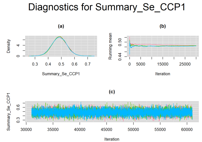
}For example, in the figure below, the posterior densities (a), running posterior mean values (b) and history plots (c) for the parameter Summary_Se_CCP1 (summary sensitivity of the first generation anti-CCP test) are displayed for each chain represented by different color. The similarity of the results from all three chains suggest the algorithm has converged to the same solution.
SUMMARY STATISTICS
Once convergence of the MCMC algorithm is achieved, summary statistics of the parameters of interest may be extracted from their posterior distributions using the MCMCsummary function found in the MCMCvis package. The datatable function found in the DT package is an optional function that we use to display the results in an interactive table.
# Summary statistics
library(MCMCvis)
library(DT)
datatable(MCMCsummary(output, round=4), extensions = 'AutoFill')
Below is the summary statistics output for the parameters shared across studies. The 50% quantile is the posterior median which is commonly used to estimate the parameter of interest. For the predicted sensitivity/specificity in a future study (Predicted_Se_CCP1, Predicted_Se_CCP2, Predicted_Se_CCP1 and Predicted_Se_CCP2) the 2.5% and 97.5% quantiles can be used to define prediction intervals for the mean sensitivity and mean specificity, respectively. If the prediction interval is much wider than the credible interval it would be indicative of presence of between-study heterogeneity in the index test.
The table also displays Rhat, which is the Gelman-Rubin statistic (Gelman and Rubin (1992), Brooks and Gelman (1998)). It is enabled when 2 or more chains are generated. It evaluates MCMC convergence by comparing within- and between-chain variability for each model parameter. Rhat tends to 1 as convergence is approached.
Also, n.eff is the effective sample size (Gelman et al. (2013)). Because the MCMC process causes the posterior draws to be correlated, the effective sample size is an estimate of the sample size required to achieve the same level of precision if that sample was a simple random sample. When draws are correlated, the effective sample size will generally be lower than the actual numbers of draws.
For instance, the summary sensitivity of CCP2 (Summary_Se_CCP2) and CCP1 (Summary_Se_CCP1) are 64.97% [95% credible interval : 2.62 , 70.34] and 37.48% [95% credible interval : 5.64 , 48.49], respectively.
The summary specificity of CCP2 (Summary_Sp_CCP2) and CCP1 (Summary_Sp_CCP1) are 93.72% [95% credible interval : 0.74 , 95.32] and 94.13% [95% credible interval : 1 , 96.56], respectively.
HETEROGENEITY
From the posterior estimates listed above, it would suggests that the sensitivity of anti-CCP assays varies according to generations, but not for specificity. We monitored the differences between those parameters in our model. The difference between both sensitivities given by parameter Difference_Se is 9.45% [95% credible interval : 6.23, 21.81]. The 95% credible interval excludes the value zero. We can therefore say that the difference is statistically significant, i.e. the summary sensitivity of second generation assays is different (and appears to be greater) than the summary sensitivity of first generation assays.
The posterior mean of the parameter Prob_Se = 0.9997. Therefore we can say there is a 0.9997 probability that the summary sensitivity of CCP2 is greater than the summary sensitivity of CCP1.
The difference between both specificities given by parameter Difference_Sp is -3.4% [95% credible interval : 1.24, -1.24]. The 95% credible interval includes the value zero. Therefore, we do not have enough evidence to conclude the summary specificity of CCP2 is different than the summary specificity of CCP1.
The posterior mean of the parameter Prob_Sp = 0.1585. Therefore we can say there is a 0.1585 probability that the summary sensitivity of CCP2 is greater than the summary sensitivity of CCP1.
We would therefore conclude our heterogeneity investigation by saying that anti-CCP test for diagnosis of rheumatoid arthritis is more likely to have a higher sensitivity for second generation assays.
RESULTS IF IGNORING HETEROGENEITY
As a comparison, if we had ignored the generation of the assays covariate by using a standard Bayesian bivariate meta-analysis model as described in this blog article we would have instead obtained a summary sensitivity (Summary_Se) of 59.98% [95% credible interval : 2.88 , 65.82] and a summary specificity (Summary_Sp) of 94.31% [95% credible interval : 0.6 , 95.62].
SCRIPT
Below is a copy of the complete script to run the Bayesian Bivariate meta-regression model in rjags.
####################################
#### DATA FOR MOTIVATING EXAMPLE ###
####################################
TP=c(115, 110, 40, 23, 236, 74, 89, 90, 31, 69, 25, 43, 70, 167, 26, 110, 26, 64, 71, 68, 38, 42, 149, 147, 47, 24, 40, 171, 72, 7, 481, 190, 82, 865, 139, 69, 90)

FP=c(17, 24, 5, 0, 20, 11, 4, 2, 0, 8, 2, 1, 5, 8, 8, 3, 1, 14, 2, 14, 3, 2, 7, 10, 7, 3, 11, 26, 14, 2, 23, 12, 13, 79, 7, 5, 7)

FN=c(16, 86, 58, 7, 88, 8, 29, 50, 22, 18, 10, 63, 17, 98, 15, 148, 20, 15, 58, 35, 0, 60, 109, 35, 20, 18, 46, 60, 77, 9, 68, 105, 71, 252, 101, 107, 101)

TN=c(73, 215, 227, 39, 231, 130, 142, 129, 75, 38, 40, 120, 228, 88, 15, 118, 56, 293, 66, 132, 73, 96, 114, 106, 375, 79, 146, 443, 298, 51, 185, 408, 301, 2218, 464, 133, 313)

Z=c(1,0,0,1,1,1,1,1,1,1,1,0,1,1,1,0,1,1,1,1,1,1,1,1,1,1,0,1,0,1,1,1,1,1,0,1,0)

pos= TP + FN
neg= TN + FP
n <- length(TP) #  Number of studies
dataList = list(TP=TP,TN=TN,n=n,pos=pos,neg=neg, Z=Z)

#################
### THE MODEL ###
#################
modelString =

  "model {
#=== LIKELIHOOD ===#
for(i in 1:n) {
TP[i] ~ dbin(se[i],pos[i])
TN[i] ~ dbin(sp[i],neg[i])
# === PRIOR FOR INDIVIDUAL LOGIT SENSITIVITY AND SPECIFICITY === #
logit(se[i]) <- l[i,1]
logit(sp[i]) <- l[i,2]
mu_reg[i,1] <- mu[1] + nu[1]*Z[i]
mu_reg[i,2] <- mu[2] + nu[2]*Z[i]
l[i,1:2] ~ dmnorm(mu_reg[i,], T[,])
}
#=== HYPER PRIOR DISTRIBUTIONS MEAN LOGIT SENSITIVITY AND SPECIFICITY === #
mu[1] ~ dnorm(0,0.3)
mu[2] ~ dnorm(0,0.3)
nu[1] ~ dnorm(0, 0.3)
nu[2] ~ dnorm(0, 0.3)

# Between-study variance-covariance matrix (TAU)
T[1:2,1:2]<-inverse(TAU[1:2,1:2])
TAU[1,1] <- tau[1]*tau[1]
TAU[2,2] <- tau[2]*tau[2]
TAU[1,2] <- rho*tau[1]*tau[2]
TAU[2,1] <- rho*tau[1]*tau[2]

#=== HYPER PRIOR DISTRIBUTIONS FOR PRECISION OF LOGIT SENSITIVITY ===#
#=== AND LOGIT SPECIFICITY, AND CORRELATION BETWEEN THEM === #
prec[1] ~ dgamma(2,0.5)
prec[2] ~ dgamma(2,0.5)
rho ~ dunif(-1,1)

# ===  PARAMETERS OF INTEREST === #

# BETWEEN-STUDY VARIANCE (tau.sq) AND STANDARD DEVIATION (tau) OF LOGIT SENSITIVITY AND SPECIFICITY
tau.sq[1]<-pow(prec[1],-1)
tau.sq[2]<-pow(prec[2],-1)
tau[1]<-pow(prec[1],-0.5)
tau[2]<-pow(prec[2],-0.5)

# SUMMARY SENSITIVITY AND SPECIFICITY OF CCP1
Summary_Se_CCP1<-1/(1+exp(-mu[1]))
Summary_Sp_CCP1<-1/(1+exp(-mu[2]))
# SUMMARY SENSITIVITY AND SPECIFICITY OF CCP2
Summary_Se_CCP2<-1/(1+exp(-mu[1] - nu[1]))
Summary_Sp_CCP2<-1/(1+exp(-mu[2] - nu[2]))
# PREDICTED SENSITIVITY AND SPECIFICITY IN A NEW STUDY EVALUATING CCP1
l_CCP1_new[1:2] ~ dmnorm(mu[],T[,])
Predicted_Se_CCP1 <- 1/(1+exp(-l_CCP1_new[1]))
Predicted_Sp_CCP1 <- 1/(1+exp(l_CCP1_new[2]))
# PREDICTED SENSITIVITY AND SPECIFICITY IN A NEW STUDY EVALUATING CCP2
mu_new[1] <- mu[1] + nu[1]
mu_new[2] <- mu[2] + nu[2]
l_CCP2_new[1:2] ~ dmnorm(mu_new[],T[,])
Predicted_Se_CCP2 <- 1/(1+exp(-l_CCP2_new[1]))
Predicted_Sp_CCP2 <- 1/(1+exp(l_CCP2_new[2]))

# POSTERIOR DIFFERENCES\ PROBABILITIES
Difference_Se <- Summary_Se_CCP2 - Summary_Se_CCP1
Difference_Sp <- Summary_Sp_CCP2 - Summary_Sp_CCP1

Prob_Se <- step(Difference_Se)
Prob_Sp <- step(Difference_Sp)
}
"

writeLines(modelString,con="model.txt")

######################
### INITIAL VALUES ###
######################
# Initial values
GenInits = function(init_mu=NULL, Seed){
  if(is.null(init_mu) == "FALSE"){
    mu = c(as.numeric(init_mu[1]),as.numeric(init_mu[2]))
  }
  else{
    mu=c(rnorm(1,0,1/sqrt(0.3)),rnorm(1,0,1/sqrt(0.3)))
  }
  list(
    mu=mu,
    nu=c(rnorm(1,0,1/sqrt(0.3)),rnorm(1,0,1/sqrt(0.3))),
    prec = c(rgamma(1,2,0.5),rgamma(1,2,0.5)),
    rho = runif(1,-1,1),
    .RNG.name="base::Wichmann-Hill",
    .RNG.seed=Seed
  )
}
seed=123
set.seed(seed)
Listinits = list(
  GenInits(init_mu=c(0,0), Seed=seed),
  GenInits(Seed=seed),
  GenInits(Seed=seed)
)

#######################################
### COMPILING AND RUNNING THE MODEL ###
#######################################
library(rjags)
# Compile the model
jagsModel = jags.model("model.txt",data=dataList,n.chains=3,inits=Listinits)
# Burn-in iterations
update(jagsModel,n.iter=300)
# Parameters to be monitored
parameters = c( "se","sp", "mu", "nu", "tau.sq", "tau", "rho",  "Summary_Se_CCP1", "Summary_Se_CCP2", "Summary_Sp_CCP1", "Summary_Sp_CCP2",  "Predicted_Se_CCP1", "Predicted_Se_CCP2", "Predicted_Sp_CCP1", "Predicted_Sp_CCP2", "Difference_Se", "Difference_Sp", "Prob_Se", "Prob_Sp")
# Posterior samples
output = coda.samples(jagsModel,variable.names=parameters,n.iter=3000)


##############################
### MONITORING CONVERGENCE ###
##############################
library(mcmcplots)
# Plots to check convergence for parameters varying across studies:
# Index j refers to the studies
# Index n refers to the number of studies
# Index i follows the ordering of the parameters vector defined in the previous box.  If left unchanged:
# i = 1: sensitivity in study j (se)
# i = 2: specificity in study j (sp)

for(j in 1:n) {
  for(i in c(1,2)) {
    #  tiff(paste(parameters[i],"[",j,"] Converged",".tiff",sep=""),width = 23, height = 23, units = "cm", res=200)
    par(oma=c(0,0,3,0))
    layout(matrix(c(1,2,3,3), 2, 2, byrow = TRUE))
    denplot(output, parms=c(paste(parameters[i],"[",j,"]",sep="")), auto.layout=FALSE, main="(a)", xlab=paste(parameters[i],"",sep=""), ylab="Density")
    rmeanplot(output, parms=c(paste(parameters[i],"[",j,"]",sep="")), auto.layout=FALSE, main="(b)")
    title(xlab="Iteration", ylab="Running mean")
    traplot(output, parms=c(paste(parameters[i],"[",j,"]",sep="")), auto.layout=FALSE, main="(c)")
    title(xlab="Iteration", ylab=paste(parameters[i],"[",j,"]",sep=""))
    mtext(paste("Diagnostics for ", parameters[i],"[",j,"]","",sep=""), side=3, line=1, outer=TRUE, cex=2)
    #  dev.off()
  }
}
# Plots to check convergence for parameters shared across studies:
# Index j = 1 refers to sensitivity and j = 2 refers to specificity
# Index i follows the ordering of the parameters vector defined above.  If left unchanged :
# i = 3 : logit-transformed mean sensitivity of index test (j=1) and logit-transformed mean specificity of index test (j=2) (mu)
# i = 4 : between-study variance in logit-transformed sensitivity of index test (j=1) and between-study variance in logit-transformed specificity of index test (j=2) (tau.sq)
# i = 5 : between-study standard deviation in logit-transformed sensitivity of index test (j=1) and between-study standard deviation in logit-transformed specificity of index test (j=2) (tau)
for(j in 1:2){
  for(i in c(3,4,5,6)) {
    #  tiff(paste(parameters[i],"[",j,"] Converged",".tiff",sep=""),width = 23, height = 23, units = "cm", res=200)
    par(oma=c(0,0,3,0))
    layout(matrix(c(1,2,3,3), 2, 2, byrow = TRUE))
    denplot(output, parms=c(paste(parameters[i],"[",j,"]",sep="")), auto.layout=FALSE, main="(a)", xlab=paste(parameters[i],"",sep=""), ylab="Density")
    rmeanplot(output, parms=c(paste(parameters[i],"[",j,"]",sep="")), auto.layout=FALSE, main="(b)")
    title(xlab="Iteration", ylab="Running mean")
    traplot(output, parms=c(paste(parameters[i],"[",j,"]",sep="")), auto.layout=FALSE, main="(c)")
    title(xlab="Iteration", ylab=paste(parameters[i],"[",j,"]",sep=""))
    mtext(paste("Diagnostics for ", parameters[i],"[",j,"]","",sep=""), side=3, line=1, outer=TRUE, cex=2)
    #  dev.off()
  }
}

# Index j not needed for the following shared parameters
# i = 6 : correlation between logit-transformed sensitivity of index test and logit-transformed specificity of index test (rho)
# i = 7 : mean sensitivity of index test (Mean_Se)
# i = 8 : mean specificity of index test (Mean_Sp)
# i = 9: predicted sensitivity of index test in a future study (Predicted_Se)
# i = 10: predicted specificity of index test in a future study (Predicted_Sp)


for(i in 7:17) {
  #  tiff(paste(parameters[i]," Converged",".tiff",sep=""),width = 23, height = 23, units = "cm", res=200)
  par(oma=c(0,0,3,0))
  layout(matrix(c(1,2,3,3), 2, 2, byrow = TRUE))
  denplot(output, parms=c(paste(parameters[i], sep="")), auto.layout=FALSE, main="(a)", xlab=paste(parameters[i],"",sep=""), ylab="Density")
  rmeanplot(output, parms=c(paste(parameters[i], sep="")), auto.layout=FALSE, main="(b)")
  title(xlab="Iteration", ylab="Running mean")
  traplot(output, parms=c(paste(parameters[i], sep="")), auto.layout=FALSE, main="(c)")
  title(xlab="Iteration", ylab=paste(parameters[i], sep=""))
  mtext(paste("Diagnostics for ", parameters[i], sep=""), side=3, line=1, outer=TRUE, cex=2)
  #  dev.off()
}

##########################
### SUMMARY STATISTICS ###
##########################
library(MCMCvis)
library(DT)
datatable(MCMCsummary(output, round=4), options = list(pageLength = 3) )
REFERENCES
Citation
@online{schiller2023,
  author = {Ian Schiller and Nandini Dendukuri},
  title = {Bayesian {Bivariate} Meta-Regression Model for Comparison of
    Summary Points},
  date = {2023-03-02},
  url = {https://www.nandinidendukuri.com/blogposts/2023-03-02-summary-points-comparison/},
  langid = {en}
}