OVERVIEW
We are often requested for the programs we have written for estimating diagnostic meta-analysis models. We felt a blog article would be a good way to share them. In this article we describe how to carry out Bayesian inference for the Bivariate meta-analysis model (Reitsma and Zwinderman (2005)).
Below we explain each step of a program in the R language (Team (2020)). The program uses the rjags package (an interface to the JAGS library (Plummer (2003)) in order to draw samples from the posterior distribution of the parameters using Markov Chain Monte Carlo (MCMC) methods. It relies on the mcmcplots package to assess convergence of the meta-analysis model. It returns summary statistics on the mean sensitivity and specificity across studies and between-study heterogeneity. A summary plot in ROC space can be created with the help of the DTAplots package.
MOTIVATING EXAMPLE AND DATA
We illustrate the script by applying it to a data from a systematic review of studies evaluating the accuracy of Anti-cyclic citrullinated peptide (Anti-CCP) test for rheumatoid arthritis (index test) compared to the 1987 revised American college or Rheumatology (ACR) criteria or clinical diagnosis (reference test) for 37 studies (Nishimura et al. (2007)). Each study provides a two-by-two table of the form
| Disease_positive | Disease_negative | |
|---|---|---|
| Inex test positive | TP | FP |
| Index test negative | FN | TN |
where:
TPis the number of individuals who tested positive on both testsFPis the number of individuals who tested positive on the index test and negative on the reference testFNis the number of individuals who tested negative on the index test and positive on the reference testTNis the number of individuals who tested negative on both tests
TP=c(115, 110, 40, 23, 236, 74, 89, 90, 31, 69, 25, 43, 70, 167, 26, 110, 26, 64, 71, 68, 38, 42, 149, 147, 47, 24, 40, 171, 72, 7, 481, 190, 82, 865, 139, 69, 90)

FP=c(17, 24, 5, 0, 20, 11, 4, 2, 0, 8, 2, 1, 5, 8, 8, 3, 1, 14, 2, 14, 3, 2, 7, 10, 7, 3, 11, 26, 14, 2, 23, 12, 13, 79, 7, 5, 7)

FN=c(16, 86, 58, 7, 88, 8, 29, 50, 22, 18, 10, 63, 17, 98, 15, 148, 20, 15, 58, 35, 0, 60, 109, 35, 20, 18, 46, 60, 77, 9, 68, 105, 71, 252, 101, 107, 101)

TN=c(73, 215, 227, 39, 231, 130, 142, 129, 75, 38, 40, 120, 228, 88, 15, 118, 56, 293, 66, 132, 73, 96, 114, 106, 375, 79, 146, 443, 298, 51, 185, 408, 301, 2218, 464, 133, 313)

pos= TP + FN
neg= TN + FP
n <- length(TP) #  Number of studies
dataList = list(TP=TP,TN=TN,n=n,pos=pos,neg=neg)
THE MODEL
Before moving any further, let’s look at a bit of theory behind the hierarchical meta-analysis model.
- Within-study level: In each study, TP is assumed to follow a Binomial distribution with probability equal to the sensitivity and TN is assumed to follow a Binomial distribution with probability equal to the specificity.
- Between-study level: The logit transformed sensitivity (\(\mu_{1i}\)) and the logit transformed specificity (\(\mu_{2i}\)) in each study jointly follow a bivariate normal distribution:
\[ \begin{pmatrix} \mu_{1i} \\ \mu_{2i} \\ \end{pmatrix} \sim N \begin{pmatrix} \begin{pmatrix} \mu_{1i} \\ \mu_{2i} \\ \end{pmatrix}, \Sigma_{12} \end{pmatrix} \text{with } \Sigma_{12} = \begin{pmatrix} \tau_{1}^2 & \rho \tau_1 \tau_2\\ \rho \tau_1 \tau_2 & \tau_2^2 \\ \end{pmatrix} \] where \(\tau_1^2\) and \(\tau_2^2\) are the between-study variance parameters and \(\rho\) is the correlation between \(\mu_{1i}\) and \(\mu_{2i}\).
The model is written in JAGS syntax, and stored in a character object that we called modelString which is later saved in the current working directory via the R function writeLines as follow.
modelString =

  "model {
#=== LIKELIHOOD ===#
for(i in 1:n) {
TP[i] ~ dbin(se[i],pos[i])
TN[i] ~ dbin(sp[i],neg[i])

# === PRIOR FOR INDIVIDUAL LOGIT SENSITIVITY AND SPECIFICITY === #
logit(se[i]) <- l[i,1]
logit(sp[i]) <- l[i,2]
l[i,1:2] ~ dmnorm(mu[], T[,])
}

#=== HYPER PRIOR DISTRIBUTIONS OVER MEAN OF LOGIT SENSITIVITY AND SPECIFICITY === #
mu[1] ~ dnorm(0,0.3)
mu[2] ~ dnorm(0,0.3)


# Between-study variance-covariance matrix (TAU)
T[1:2,1:2]<-inverse(TAU[1:2,1:2])
TAU[1,1] <- tau[1]*tau[1]
TAU[2,2] <- tau[2]*tau[2]
TAU[1,2] <- rho*tau[1]*tau[2]
TAU[2,1] <- rho*tau[1]*tau[2]

#=== HYPER PRIOR DISTRIBUTIONS FOR PRECISION OF LOGIT SENSITIVITY ===#
#=== AND LOGIT SPECIFICITY, AND CORRELATION BETWEEN THEM === #
prec[1] ~ dgamma(2,0.5)
prec[2] ~ dgamma(2,0.5)
rho ~ dunif(-1,1)

# ===  PARAMETERS OF INTEREST === #
# BETWEEN-STUDY VARIANCE (tau.sq) AND STANDARD DEVIATION (tau) OF LOGIT SENSITIVITY AND SPECIFICITY
tau.sq[1]<-pow(prec[1],-1)
tau.sq[2]<-pow(prec[2],-1)
tau[1]<-pow(prec[1],-0.5)
tau[2]<-pow(prec[2],-0.5)
# MEAN SENSITIVITY AND SPECIFICITY
Summary_Se <- 1/(1+exp(-mu[1]))
Summary_Sp <- 1/(1+exp(-mu[2]))

# PREDICTED SENSITIVITY AND SPECIFICITY IN A NEW STUDY
l.predicted[1:2] ~ dmnorm(mu[],T[,])
Predicted_Se <- 1/(1+exp(-l.predicted[1]))
Predicted_Sp <- 1/(1+exp(-l.predicted[2]))
}"

writeLines(modelString,con="model.txt")
INTIAL VALUES
Running multiple chains, each starting at different initial values, serves to assess convergence of the MCMC algorithm by examining if all chains reach the same solution. There are different ways of providing initial values. In the illustration below we give details on how to provide initial values chosen by the user by using a homemade function we are calling GenInits().
Providing relevant initial values can speed up convergence of the MCMC algorithm. Here we create a function that allows us to provide our own initial values for the logit-transformed sensitivity (mu[1]) and logit-transformed specificity (mu[2]) parameters. We can provide specific initial values to mu[1] and mu[2] through the init_mu argument or we can use the function to randomly generate initial values from a normal distribution (corresponding to the prior distribution found in the model) for mu[1] and mu[2]. In this example, we have allowed other parameters, such as between-study precisions (prec[1] and prec[2]) and correlation between logit-transformed sensitivity and logit-transformed specificity (rho) to be randomly generated by GenInits(). In our experience, choosing initial values for these parameters is not easy. For reproducibility, a Seed argument is provided.
In the illustration below, we set mu[1] and mu[2] equal to 0 (which represents an initial value of 0.5 on the probability scale)for the first chain. For chains number 2 and 3, we simply set the argument init_mu to NULL. This ensures both chain 2 and chain 3 are randomly initialized.
# Initial values
GenInits = function(init_mu=NULL, Seed){
  if(is.null(init_mu) == "FALSE"){
    mu = c(as.numeric(init_mu[1]),as.numeric(init_mu[2]))
  }
  else{
    mu=c(rnorm(1,0,1/sqrt(0.3)),rnorm(1,0,1/sqrt(0.3)))
  }
  list(
    mu=mu,
    prec = c(rgamma(1,2,0.5),rgamma(1,2,0.5)),
    rho = runif(1,-1,1),
    .RNG.name="base::Wichmann-Hill",
    .RNG.seed=Seed
  )
}
seed=123
set.seed(seed)
Listinits = list(
  GenInits(init_mu=c(0,0), Seed=seed),
  GenInits(Seed=seed),
  GenInits(Seed=seed)
)
COMPILING AND RUNNING THE MODEL
The jags.model function compiles the model for possible syntax errors. Argument n.chains=3 creates 3 MCMC chains with different starting values given by the Listinits object defined above.
library(rjags)
# Compile the model
jagsModel = jags.model("model.txt",data=dataList,n.chains=3,inits=Listinits)
The update function serves as to carry out the “burn-in” step. This corresponds to discarding initial iterations till the MCMC algorithm has reached its equilibrium distribution. Here we chose to discard 30,000 iterations by providing argument n.iter=30000. This can be helpful to mitigate “bad” initial values.
# Burn-in iterations
update(jagsModel,n.iter=30000)
The coda.samples function draws samples from the posterior distribution of the unknown parameters that were defined in the parameters object. Here we are drawing n.iter=30000 iterations from the posterior distributions for each chain.
# Parameters to be monitored
parameters = c( "se","sp", "mu", "tau.sq", "tau", "rho",  "Summary_Se", "Summary_Sp",  "Predicted_Se", "Predicted_Sp")

# Posterior samples
output = coda.samples(jagsModel,variable.names=parameters,n.iter=30000)
MONITORING CONVERGENCE
Convergence of the MCMC algorithm can now be examined. The code below will create a 3-panel plot consisting of the density plot, the running mean plot and a history plot for parameters that vary across studies, e.g. prevalence, sensitivity and specificity in each study.
library(mcmcplots)
# Plots to check convergence for parameters varying across studies:
# Index j refers to the studies
# Index n refers to the number of studies
# Index i follows the ordering of the parameters vector defined in the previous box.  If left unchanged:
# i = 1: sensitivity in study j (se)
# i = 2: specificity in study j (sp)

for(j in 1:n) {
for(i in c(1,2)) {
  #  tiff(paste(parameters[i],"[",j,"] Converged",".tiff",sep=""),width = 23, height = 23, units = "cm", res=200)
  par(oma=c(0,0,3,0))
  layout(matrix(c(1,2,3,3), 2, 2, byrow = TRUE))
  denplot(output, parms=c(paste(parameters[i],"[",j,"]",sep="")), auto.layout=FALSE, main="(a)", xlab=paste(parameters[i],"",sep=""), ylab="Density")
  rmeanplot(output, parms=c(paste(parameters[i],"[",j,"]",sep="")), auto.layout=FALSE, main="(b)")
  title(xlab="Iteration", ylab="Running mean")
  traplot(output, parms=c(paste(parameters[i],"[",j,"]",sep="")), auto.layout=FALSE, main="(c)")
  title(xlab="Iteration", ylab=paste(parameters[i],"[",j,"]",sep=""))
  mtext(paste("Diagnostics for ", parameters[i],"[",j,"]","",sep=""), side=3, line=1, outer=TRUE, cex=2)
  #  dev.off()
}
}
Then we create the same 3-panel plot for the parameters that are shared across studies.
# Plots to check convergence for parameters shared across studies:
# Index j = 1 refers to sensitivity and j = 2 refers to specificity
# Index i follows the ordering of the parameters vector defined above. If left unchanged :
# i = 3 : logit-transformed mean sensitivity of index test (j=1) and logit-transformed mean specificity of index test (j=2) (mu)
# i = 4 : between-study variance in logit-transformed sensitivity of index test (j=1) and between-study variance in logit-transformed specificity of index test (j=2) (tau.sq)
# i = 5 : between-study standard deviation in logit-transformed sensitivity of index test (j=1) and between-study standard deviation in logit-transformed specificity of index test (j=2) (tau)
for(j in 1:2){
for(i in c(3,4,5)) {
# tiff(paste(parameters[i],"[",j,"] Converged",".tiff",sep=""),width = 23, height = 23, units = "cm", res=200)
par(oma=c(0,0,3,0))
layout(matrix(c(1,2,3,3), 2, 2, byrow = TRUE))
denplot(output, parms=c(paste(parameters[i],"[",j,"]",sep="")), auto.layout=FALSE, main="(a)", xlab=paste(parameters[i],"",sep=""), ylab="Density")
rmeanplot(output, parms=c(paste(parameters[i],"[",j,"]",sep="")), auto.layout=FALSE, main="(b)")
title(xlab="Iteration", ylab="Running mean")
traplot(output, parms=c(paste(parameters[i],"[",j,"]",sep="")), auto.layout=FALSE, main="(c)")
title(xlab="Iteration", ylab=paste(parameters[i],"[",j,"]",sep=""))
mtext(paste("Diagnostics for ", parameters[i],"[",j,"]","",sep=""), side=3, line=1, outer=TRUE, cex=2)
# dev.off()
}
}
# Index j not needed for the following shared parameters
# i = 6 : correlation between logit-transformed sensitivity of index test and logit-transformed specificity of index test (rho)
# i = 7 : mean sensitivity of index test (Mean_Se)
# i = 8 : mean specificity of index test (Mean_Sp)
# i = 9: predicted sensitivity of index test in a future study (Predicted_Se)
# i = 10: predicted specificity of index test in a future study (Predicted_Sp)
for(i in 6:10) {
# tiff(paste(parameters[i]," Converged",".tiff",sep=""),width = 23, height = 23, units = "cm", res=200)
par(oma=c(0,0,3,0))
layout(matrix(c(1,2,3,3), 2, 2, byrow = TRUE))
denplot(output, parms=c(paste(parameters[i], sep="")), auto.layout=FALSE, main="(a)", xlab=paste(parameters[i],"",sep=""), ylab="Density")
rmeanplot(output, parms=c(paste(parameters[i], sep="")), auto.layout=FALSE, main="(b)")
title(xlab="Iteration", ylab="Running mean")
traplot(output, parms=c(paste(parameters[i], sep="")), auto.layout=FALSE, main="(c)")
title(xlab="Iteration", ylab=paste(parameters[i], sep=""))
mtext(paste("Diagnostics for ", parameters[i], sep=""), side=3, line=1, outer=TRUE, cex=2)
# dev.off()
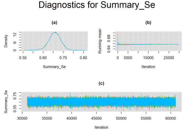
}For example, in the figure below, the posterior densities (a), running posterior mean values (b) and history plots (c) for the parameter Summary_Se (summary sensitivity of the Anti-CCP test) are displayed for each chain represented by different color. The similar results from all five chains suggest the algorithm has converged to the same solution in each case.
SUMMARY STATISTICS
Once convergence of the MCMC algorithm is achieved, summary statistics of the parameters of interest may be extracted from their posterior distributions using the MCMCsummary function found in the MCMCvis package.
# Summary statistics
library(DT)
datatable(output, extensions = 'AutoFill', options = list(autoFill = TRUE))
Below is the summary statistics output for the parameters shared across studies. The 50% quantile is the posterior median which is commonly used to estimate the paramater of interest. The 2.5% and 97.5% quantiles for the Predicted_Se and Predicted_Sp can be used to define prediction intervals for the mean sensitivity and mean specificity, respectively. If the prediction interval is much wider than the credible interval it would be indicative of high between-study heterogeneity in the index test.
The table also displays Rhat, which is the Gelman-Rubin statistic (Gelman and Rubin (1992), Brooks and Gelman (1998)). It is enabled when 2 or more chains are generated. It evaluates MCMC convergence by comparing within- and between-chain variability for each model parameter. Rhat tends to 1 as convergence is approached.
Also, n.eff is the effective sample size (Gelman et al. (2013)). Because the MCMC process causes the posterior draws to be correlated, the effective sample size is an estimate of the sample size required to achieve the same level of precision if that sample was a simple random sample. When draws are correlated, the effective sample size will generally be lower than the actual numbers of draws.
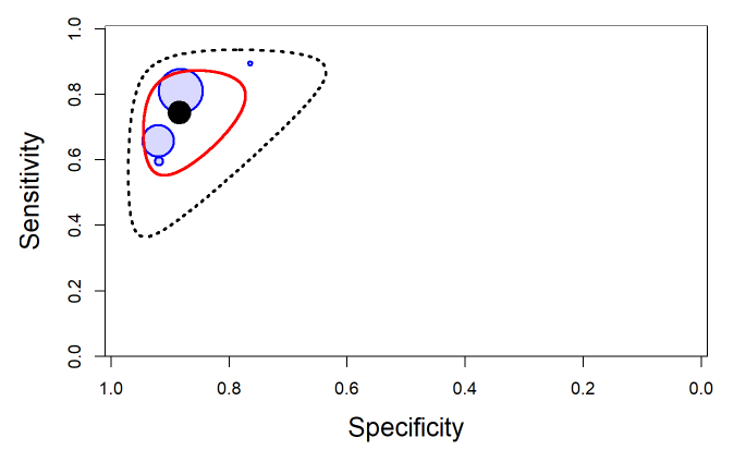
SROC PLOT
The output from rjags can be used to obtain a plot in the summary receiver operating characteristic (SROC) space with 95% credible region (red line) and 95% prediction region (black dotted line) around the summary estimates of sensitivity and specificity (solid black circle) using the SROC_rjags function found in the DTAplots package. Individual studies can also be represented (blue circles) and are proportional to their sample size. The argument ref_std=TRUEis required to allow the plot to reflect the assumption of a perfect reference test.
# SROC plot
library(DTAplots)
SROC_rjags(X=output, model="Bivariate",n=n, study_col1="blue", study_col2=rgb(0, 0, 1, 0.15), dataset=cbind(TP,FP,FN,TN), ref_std=TRUE, Sp.range=c(0,1))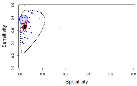
SCRIPT
Below is a copy of the complete script to run the Bayesian Bivariate meta-analysis model in rjags.
####################################
#### DATA FOR MOTIVATING EXAMPLE ###
####################################
TP=c(115, 110, 40, 23, 236, 74, 89, 90, 31, 69, 25, 43, 70, 167, 26, 110, 26, 64, 71, 68, 38, 42, 149, 147, 47, 24, 40, 171, 72, 7, 481, 190, 82, 865, 139, 69, 90)

FP=c(17, 24, 5, 0, 20, 11, 4, 2, 0, 8, 2, 1, 5, 8, 8, 3, 1, 14, 2, 14, 3, 2, 7, 10, 7, 3, 11, 26, 14, 2, 23, 12, 13, 79, 7, 5, 7)

FN=c(16, 86, 58, 7, 88, 8, 29, 50, 22, 18, 10, 63, 17, 98, 15, 148, 20, 15, 58, 35, 0, 60, 109, 35, 20, 18, 46, 60, 77, 9, 68, 105, 71, 252, 101, 107, 101)

TN=c(73, 215, 227, 39, 231, 130, 142, 129, 75, 38, 40, 120, 228, 88, 15, 118, 56, 293, 66, 132, 73, 96, 114, 106, 375, 79, 146, 443, 298, 51, 185, 408, 301, 2218, 464, 133, 313)

pos= TP + FN
neg= TN + FP
n <- length(TP) #  Number of studies
dataList = list(TP=TP,TN=TN,n=n,pos=pos,neg=neg)

#################
### THE MODEL ###
#################
modelString =

  "model {
#=== LIKELIHOOD ===#
for(i in 1:n) {
TP[i] ~ dbin(se[i],pos[i])
TN[i] ~ dbin(sp[i],neg[i])

# === PRIOR FOR INDIVIDUAL LOGIT SENSITIVITY AND SPECIFICITY === #
logit(se[i]) <- l[i,1]
logit(sp[i]) <- l[i,2]
l[i,1:2] ~ dmnorm(mu[], T[,])
}

#=== HYPER PRIOR DISTRIBUTIONS OVER MEAN OF LOGIT SENSITIVITY AND SPECIFICITY === #
mu[1] ~ dnorm(0,0.3)
mu[2] ~ dnorm(0,0.3)

# Between-study variance-covariance matrix (TAU)
T[1:2,1:2]<-inverse(TAU[1:2,1:2])
TAU[1,1] <- tau[1]*tau[1]
TAU[2,2] <- tau[2]*tau[2]
TAU[1,2] <- rho*tau[1]*tau[2]
TAU[2,1] <- rho*tau[1]*tau[2]

#=== HYPER PRIOR DISTRIBUTIONS FOR PRECISION OF LOGIT SENSITIVITY ===#
#=== AND LOGIT SPECIFICITY, AND CORRELATION BETWEEN THEM === #
prec[1] ~ dgamma(2,0.5)
prec[2] ~ dgamma(2,0.5)
rho ~ dunif(-1,1)

# ===  PARAMETERS OF INTEREST === #
# BETWEEN-STUDY VARIANCE (tau.sq) AND STANDARD DEVIATION (tau) OF LOGIT SENSITIVITY AND SPECIFICITY
tau.sq[1]<-pow(prec[1],-1)
tau.sq[2]<-pow(prec[2],-1)
tau[1]<-pow(prec[1],-0.5)
tau[2]<-pow(prec[2],-0.5)
# MEAN SENSITIVITY AND SPECIFICITY
Summary_Se <- 1/(1+exp(-mu[1]))
Summary_Sp <- 1/(1+exp(-mu[2]))

# PREDICTED SENSITIVITY AND SPECIFICITY IN A NEW STUDY
l.predicted[1:2] ~ dmnorm(mu[],T[,])
Predicted_Se <- 1/(1+exp(-l.predicted[1]))
Predicted_Sp <- 1/(1+exp(-l.predicted[2]))
}"

writeLines(modelString,con="model.txt")

######################
### INITIAL VALUES ###
######################
GenInits = function(init_mu=NULL, Seed){
  if(is.null(init_mu) == "FALSE"){
    mu = c(as.numeric(init_mu[1]),as.numeric(init_mu[2]))
  }
  else{
    mu=c(rnorm(1,0,1/sqrt(0.3)),rnorm(1,0,1/sqrt(0.3)))
  }
  list(
    mu=mu,
    prec = c(rgamma(1,2,0.5),rgamma(1,2,0.5)),
    rho = runif(1,-1,1),
    .RNG.name="base::Wichmann-Hill",
    .RNG.seed=Seed
  )
}
seed=123
set.seed(seed)
Listinits = list(
  GenInits(init_mu=c(0,0), Seed=seed),
  GenInits(Seed=seed),
  GenInits(Seed=seed)
)

#######################################
### COMPILING AND RUNNING THE MODEL ###
#######################################
library(rjags)
jagsModel = jags.model("model.txt",data=dataList,n.chains=3,inits=Listinits)
# Burn-in iterations
update(jagsModel,n.iter=30000)
# Parameters to be monitored
parameters = c( "se","sp", "mu", "tau.sq", "tau", "rho",  "Summary_Se", "Summary_Sp",  "Predicted_Se", "Predicted_Sp")
# Posterior samples
output = coda.samples(jagsModel,variable.names=parameters,n.iter=30000)


##############################
### MONITORING CONVERGENCE ###
##############################
library(mcmcplots)
# Plots to check convergence for parameters varying across studies:
# Index j refers to the studies
# Index n refers to the number of studies
# Index i follows the ordering of the parameters vector defined in the previous box.  If left unchanged:
# i = 1: sensitivity in study j (se)
# i = 2: specificity in study j (sp)

for(j in 1:n) {
for(i in c(1,2)) {
  #  tiff(paste(parameters[i],"[",j,"] Converged",".tiff",sep=""),width = 23, height = 23, units = "cm", res=200)
  par(oma=c(0,0,3,0))
  layout(matrix(c(1,2,3,3), 2, 2, byrow = TRUE))
  denplot(output, parms=c(paste(parameters[i],"[",j,"]",sep="")), auto.layout=FALSE, main="(a)", xlab=paste(parameters[i],"",sep=""), ylab="Density")
  rmeanplot(output, parms=c(paste(parameters[i],"[",j,"]",sep="")), auto.layout=FALSE, main="(b)")
  title(xlab="Iteration", ylab="Running mean")
  traplot(output, parms=c(paste(parameters[i],"[",j,"]",sep="")), auto.layout=FALSE, main="(c)")
  title(xlab="Iteration", ylab=paste(parameters[i],"[",j,"]",sep=""))
  mtext(paste("Diagnostics for ", parameters[i],"[",j,"]","",sep=""), side=3, line=1, outer=TRUE, cex=2)
  #  dev.off()
}
}
# Plots to check convergence for parameters shared across studies:
# Index j = 1 refers to sensitivity and j = 2 refers to specificity
# Index i follows the ordering of the parameters vector defined above.  If left unchanged :
# i = 3 : logit-transformed mean sensitivity of index test (j=1) and logit-transformed mean specificity of index test (j=2) (mu)
# i = 4 : between-study variance in logit-transformed sensitivity of index test (j=1) and between-study variance in logit-transformed specificity of index test (j=2) (tau.sq)
# i = 5 : between-study standard deviation in logit-transformed sensitivity of index test (j=1) and between-study standard deviation in logit-transformed specificity of index test (j=2) (tau)
for(j in 1:2){
for(i in c(3,4,5)) {
  #  tiff(paste(parameters[i],"[",j,"] Converged",".tiff",sep=""),width = 23, height = 23, units = "cm", res=200)
  par(oma=c(0,0,3,0))
  layout(matrix(c(1,2,3,3), 2, 2, byrow = TRUE))
  denplot(output, parms=c(paste(parameters[i],"[",j,"]",sep="")), auto.layout=FALSE, main="(a)", xlab=paste(parameters[i],"",sep=""), ylab="Density")
  rmeanplot(output, parms=c(paste(parameters[i],"[",j,"]",sep="")), auto.layout=FALSE, main="(b)")
  title(xlab="Iteration", ylab="Running mean")
  traplot(output, parms=c(paste(parameters[i],"[",j,"]",sep="")), auto.layout=FALSE, main="(c)")
  title(xlab="Iteration", ylab=paste(parameters[i],"[",j,"]",sep=""))
  mtext(paste("Diagnostics for ", parameters[i],"[",j,"]","",sep=""), side=3, line=1, outer=TRUE, cex=2)
  #  dev.off()
}
}

# Index j not needed for the following shared parameters
# i = 6 : correlation between logit-transformed sensitivity of index test and logit-transformed specificity of index test (rho)
# i = 7 : mean sensitivity of index test (Mean_Se)
# i = 8 : mean specificity of index test (Mean_Sp)
# i = 9: predicted sensitivity of index test in a future study (Predicted_Se)
# i = 10: predicted specificity of index test in a future study (Predicted_Sp)


for(i in 6:10) {
  #  tiff(paste(parameters[i]," Converged",".tiff",sep=""),width = 23, height = 23, units = "cm", res=200)
  par(oma=c(0,0,3,0))
  layout(matrix(c(1,2,3,3), 2, 2, byrow = TRUE))
  denplot(output, parms=c(paste(parameters[i], sep="")), auto.layout=FALSE, main="(a)", xlab=paste(parameters[i],"",sep=""), ylab="Density")
  rmeanplot(output, parms=c(paste(parameters[i], sep="")), auto.layout=FALSE, main="(b)")
  title(xlab="Iteration", ylab="Running mean")
  traplot(output, parms=c(paste(parameters[i], sep="")), auto.layout=FALSE, main="(c)")
  title(xlab="Iteration", ylab=paste(parameters[i], sep=""))
  mtext(paste("Diagnostics for ", parameters[i], sep=""), side=3, line=1, outer=TRUE, cex=2)
  #  dev.off()
}

##########################
### SUMMARY STATISTICS ###
##########################
library(MCMCvis)
library(DT)
datatable(MCMCsummary(output, round=4), options = list(pageLength = 3) )

#################
### SROC PLOT ###
#################
library(DTAplots)
SROC_rjags(X=output, model="Bivariate",n=n, study_col1="blue", study_col2=rgb(0, 0, 1, 0.15), dataset=cbind(TP,FP,FN,TN), ref_std=TRUE, Sp.range=c(0,1))
REFERENCES
Citation
@online{schiller2021,
  author = {Ian Schiller and Nandini Dendukuri},
  title = {Bayesian Inference for the {Bivariate} Model for Diagnostic
    Meta-Analysis},
  date = {2021-04-13},
  url = {https://www.nandinidendukuri.com/blogposts/2021-04-13-bayesian-bivariate-meta-analysis/},
  langid = {en}
}