OVERVIEW
This is a second article in our series of blog articles illustrating Rjags programs for diagnostic meta-analysis models. We previously looked at the Bayesian bivariate model. In this article we describe how to carry out Bayesian inference for the Bivariate latent class meta-analysis model (Xie, Sinclair and Dendukuri Xie, Sinclair, and Dendukuri (2017)) when a perfect reference test is not available.
This blog will guide you through each step of a program in the R language (R Core Team Team (2020)). The program uses the rjags package (an interface to the JAGS library (Plummer Plummer (2003) ) in order to draw samples from the posterior distribution of the parameters using Markov Chain Monte Carlo (MCMC) methods. The program relies on the mcmcplots package to assess convergence of the meta-analysis model. It returns summary statistics on the mean sensitivity and specificity across studies and between-study heterogeneity. A summary plot in ROC space can be created with the help of the DTAplots package.
MOTIVATING EXAMPLE AND DATA
To illustrate the method, we apply the script to a data from a systematic review of studies evaluating the accuracy of GeneXpertTM (Xpert) test for tuberculosis (TB) meningitis (index test) and culture (reference test) for 29 studies (Kohli et al Kohli et al. (2018) ). Each study provides a two-by-two table of the form
| reference_test_positive | Reference_test_negative | |
|---|---|---|
| Index test positive | t11 | t10 |
| Index test negative | t01 | t00 |
where:
t11is the number of individuals who tested positive on both Xpert and culture testst10is the number of individuals who tested positive on Xpert and negative on culture testt01is the number of individuals who tested negative on Xpert and positive on culture testt00is the number of individuals who tested negative on both Xpert and culture tests
t11 <- c(7, 6, 2, 5, 0, 1, 4, 3, 3, 1, 7, 35, 103, 1, 2, 22, 6, 25, 27, 15, 5, 2, 2, 11, 2, 0, 8, 3, 1)
t10 <- c(5, 4, 0, 0, 0, 0, 6, 0, 3, 0, 0, 5, 6, 1, 0, 1, 1, 3, 11, 3, 9, 3, 0, 2, 4, 0, 2, 0, 2)
t01 <- c(5, 4, 0, 1, 2, 0, 8, 1, 1, 0, 0, 1, 18, 2, 0, 5, 0, 20, 25, 7, 10, 1, 1, 2, 2, 3, 5, 0, 0)
t00 <- c(63, 115, 2, 44, 132, 4, 83, 250, 67, 14, 150, 119, 252, 107, 8, 31, 148, 687, 204, 205, 115, 53, 4, 118, 22, 16, 186, 28, 43)
cell <- cbind(t11, t10, t01, t00)
n <- length(t11)  #  Number of studies
n.study <- rowSums(cell) #  Study sample sizes
dataList <- list(t12=cell,n=n, n.study=n.study)
THE MODEL
Before moving any further, let’s look at a bit of theory behind the latent class meta-analysis model. In a latent class model, the target condition is assumed unknown.
**Within-study level:** In each study, the entries of the 2x2 table defined in the previous section are assumed to follow a multinomial distribution with probabilities ``p11``, ``p10``, ``p01`` and ``p00`` expressed as follows :
\[ (t11, t10, t01, t00) \sim \text{Multinomial}((p11, p10, p01, p00), n.study) \]
where
\[p11 = prev*(se1*se2 + covp) + (1-prev)*((1-sp1)*(1-sp2) + covn)\]
\[ p10 = prev*(se1*(1-se2) - covp) + (1-prev)*((1-sp1)*sp2 - covn)\]
\[ p01 = prev*((1-se1)*se2 - covp)$ + (1-prev)*(sp1*(1-sp2) - covn) \]
\[p00 = prev*((1-se1)*(1-se2) + covp) + (1-prev)*(sp1*sp2 + covn)\]
\[-(1-s1)*(1-s2) < covp < max(s1,s2) – s1*s2\]
\[-(1-c1)*(1-c2) < covn < max(c1,c2) – c1*c2\]
where prev denotes the prevalence of the latent target condition, se1 and sp1 denote the sensitivity and specificity of the index test, se2 and sp2 denote the sensitivity and specificity of the reference test, covp`is the covariance between the tests among those who have the target condition, covn is the covariance between the tests among those who do not have the target condition and n.study is the total sample size in all four cells. The covariance terms adjust for the possibility that both tests make the same false positive or false negative errors. This is referred to as conditional dependence.
Between-study level: For the index test, the logit transformed sensitivity ( \(\mu_{1i}\)) and the logit transformed specificity (\(\mu_{1i}\) ) in each study jointly follow a bivariate normal distribution:
\[ \begin{pmatrix} \mu_{1i} \\ \mu_{2i} \\ \end{pmatrix} \sim N \begin{pmatrix} \begin{pmatrix} \mu_{1i} \\ \mu_{2i} \\ \end{pmatrix}, \Sigma_{12} \end{pmatrix} \text{with } \Sigma_{12} = \begin{pmatrix} \tau_{1}^2 & \rho \tau_1 \tau_2\\ \rho \tau_1 \tau_2 & \tau_2^2 \\ \end{pmatrix} \] where \(\tau_1^2\) and \(\tau_2^2\) are the between-study variance parameters and \(\rho\) is the correlation between \(\mu_{1i}\) and \(\mu_{2i}\).
To carry out Bayesian estimation, we need to specify prior distribution over the unknown parameters. A hierarchical prior distribution structure is specified for the sensitivity and specificity of the index test to account for both between- and within-study variability and the correlation between the sensitivity and specificity across studies. A similar hierarchical prior distribution is specified over the sensitivity and specificity of the reference standard. Additionally, prior distributions must be specified for the prevalence in each study and for the covariance parameters.
The model is written in JAGS syntax, and stored in a character object that we called modelString which is later saved in the current working directory via the R function writeLines as follow.
# Bayesian bivariate latent class model
modelString =
  "model {

#=== LIKELIHOOD ===#
for(i in 1:n) {

t12[i,1:4] ~ dmulti(p12[i,1:4],n.study[i])

p12[i,1] <- prev[i]*( se[i]* se2[i]     +covp[i]) + (1-prev[i])*( (1-sp[i])*(1-sp2[i]) +covn[i])
p12[i,2] <- prev[i]*( se[i]* (1-se2[i]) -covp[i]) + (1-prev[i])*( (1-sp[i])*sp2[i]     -covn[i])
p12[i,3] <- prev[i]*( (1-se[i])*se2[i]     -covp[i]) + (1-prev[i])*( sp[i]*(1-sp2[i]) -covn[i])
p12[i,4] <- prev[i]*( (1-se[i])*(1-se2[i]) +covp[i]) + (1-prev[i])*( sp[i]*sp2[i] +covn[i])


# Hierarchical prior distribution for XPERT test
logit(se[i]) <- l[i,1]
logit(sp[i]) <- l[i,2]
l[i,1:2] ~ dmnorm(mu[1:2], T[1:2,1:2])

# Hierarchical prior distribution for CUTURE test
logit(se2[i]) <- l2[i,1]
logit(sp2[i]) <- l2[i,2]
l2[i,1:2] ~ dmnorm(mu2[1:2],T2[1:2,1:2])

# Prior distribution for prevalence
prev[i] ~ dbeta(1,1)

#=== CONDITIONAL DEPENDENCE STRUCTURE ===#
# lower and upper limits of covariance parameters
maxs12[i]<-min(se[i],se2[i])-(se[i]*se2[i])
maxc12[i]<-min(sp[i],sp2[i])-(sp[i]*sp2[i])
mins12[i]<- (1-se[i])*(se2[i]-1)
minc12[i]<- (1-sp[i])*(sp2[i]-1)

# covariance parameters
covp[i] ~ dunif(mins12[i], maxs12[i]);
covn[i] ~ dunif(minc12[i], maxc12[i]);
}

####    HYPER PRIOR DISTRIBUTIONS FOR XPERT ACCURACY    ####
# prior for the logit transformed sensitivity (mu[1]) and logit transformed  specificity (mu[2]) of XPERT test
mu[1] ~ dnorm(0,0.3)
mu[2] ~ dnorm(0,0.3)

# Between-study variance-covariance matrix of XPERT test
T[1:2,1:2]<-inverse(TAU[1:2,1:2])
TAU[1,1] <- tau[1]*tau[1]
TAU[2,2] <- tau[2]*tau[2]
TAU[1,2] <- rho*tau[1]*tau[2]
TAU[2,1] <- rho*tau[1]*tau[2]

# prior for the between-study precision of the logit transformed sensitivity (prec[1]) and logit transformed specificity (prec[2]) of XPERT test
prec[1] ~ dgamma(2,0.5)
prec[2] ~ dgamma(2,0.5)
rho ~ dunif(-1,1)

####    HYPER PRIOR DISTRIBUTIONS FOR CULTURE ACCURACY    ####
# prior for the logit transformed sensitivity (mu[1]) and logit transformed  specificity (mu[2]) of CULTURE test
mu2[1] ~ dnorm(0,0.3)
mu2[2] ~ dnorm(0,0.3)

# Between-study variance-covariance matrix of CULTURE test
T2[1:2,1:2] <- inverse(TAU2[1:2,1:2])
TAU2[1,1] <- tau2[1]*tau2[1]
TAU2[2,2] <- tau2[2]*tau2[2]
TAU2[1,2] <- rho2*tau2[1]*tau2[2]
TAU2[2,1] <- rho2*tau2[1]*tau2[2]

# prior for the between-study precision of the logit transformed sensitivity (prec2[1]) and logit transformed specificity (prec2[2]) of CULTURE test
prec2[1] ~ dgamma(2,0.5)
prec2[2] ~ dgamma(2,0.5)
rho2 ~ dunif(-1,1)

####  OTHER PARAMETERS OF INTEREST

# Between-study standard deviation of the logit transformed sensitivity (tau[1]) and specificity (tau[2]) of XPERT test
tau[1]<-pow(prec[1],-0.5)
tau[2]<-pow(prec[2],-0.5)
tau.sq[1]<-pow(prec[1],-1)
tau.sq[2]<-pow(prec[2],-1)

# Between-study standard deviation of the logit transformed sensitivity (tau2[1]) and specificity (tau2[2]) of CULTURE test
tau2[1] <- pow(prec2[1],-0.5)
tau2[2] <- pow(prec2[2],-0.5)

# Mean sensitivity and mean specificity of XPERT
Summary_Se <-1/(1+exp(-mu[1]))
Summary_Sp <-1/(1+exp(-mu[2]))

# Predicted sensitivity and predicted specificity of XPERT in a future study
l.predict[1:2] ~ dmnorm(mu[],T[,])
Predicted_Se <- 1/(1+exp(-l.predict[1]))
Predicted_Sp <- 1/(1+exp(-l.predict[2]))

# Mean sensitivity and mean specificity of CULTURE
Summary_Se2<-1/(1+exp(-mu2[1]))
Summary_Sp2<-1/(1+exp(-mu2[2]))

# Predicted sensitivity and predicted specificity of CULTURE in a future study
l.predict2[1:2] ~ dmnorm(mu2[],T2[,])
Predicted.Se2 <- 1/(1+exp(-l.predict2[1]))
Predicted.Sp2 <- 1/(1+exp(-l.predict2[2]))
}"

writeLines(modelString,con="model.txt")
INTIAL VALUES
Running multiple chains, each starting at different initial values, serves to assess convergence of the MCMC algorithm by examining if all chains reach the same solution. There are different ways of providing initial values. In the illustration below we give details on how to provide initial values chosen by the user by using a homemade function we are calling GenInits().
Providing relevant initial values can speed up convergence of the MCMC algorithm. Here we create a function that allows us to provide our own initial values for the logit-transformed sensitivity (mu[1]) and logit-transformed specificity (mu[2]) of the test under evaluation, as well as the logit-transformed sensitivity (mu2[1]) and logit-transformed specificity (mu2[2]) of the reference test. We can provide specific initial values to mu[1], mu[2] and mu2[1], mu2[2] through the init_mu and init_mu2 arguments respectively or we can use the function to randomly generate initial values from distributions corresponding to the prior distribution found in the model for mu[1], mu[2], mu2[1] and mu2[2]. In this example, we have allowed other parameters, such as between-study precisions (prec[1] and prec[2] for test under evaluation and prec2[1] and prec2[2] for reference test), study prevalence of the latent target condition (prev[i], for i=1, …, n) and correlation between logit-transformed sensitivity and logit-transformed specificity (rho for test under evaluation rho2 for reference test), to be randomly generated by GenInits(). In our experience, choosing initial values for these parameters is not easy. Initial values for the covariance between the tests (covp among those who have the target condition and covn among those who do not have the target condition) are initialised to be equal to zero. For reproducibility, a Seed argument is provided.
In the illustration below, for the first chain, we set mu[1], mu[2] and mu2[1] equal to 0 (which represents an initial value of 0.5 on the probability scale) while mu2[2]=4, representing a value of 98.2% on the probability scale. For chains number 2, 3, 4 and 5, we simply set the arguments init_mu and init_mu2 to NULL respectively. This ensure the remaining 4 chains are randomly initialized. The number of studies n, must also be provided as an argument to the function.
# Initial values
GenInits = function(init_mu=NULL, init_mu2=NULL, Seed=seed, n){
  if(is.null(init_mu) == FALSE & is.null(init_mu2) == FALSE){
    mu = c(as.numeric(init_mu[1]),as.numeric(init_mu[2]))
    mu2 = c(as.numeric(init_mu2[1]),as.numeric(init_mu2[2]))
  }
  else{
    mu=c(rnorm(1,0,1/sqrt(0.3)),rnorm(1,0,1/sqrt(0.3)))
    mu2=c(rnorm(1,0,1/sqrt(0.3)),rnorm(1,0,1/sqrt(0.3)))
  }
  list(
    mu=mu,
    mu2=mu2,
    covn = rep(0,n),
    covp = rep(0,n),
    prev = runif(n),
    prec = c(rgamma(1,2,0.5),rgamma(1,2,0.5)),
    prec2 = c(rgamma(1,2,0.5),rgamma(1,2,0.5)),
    rho = runif(1,-1,1),
    rho2 = runif(1,-1,1) ,
    .RNG.name="base::Wichmann-Hill",
    .RNG.seed=Seed
  )
}
seed=24050; set.seed(seed)
Listinits = list(
  GenInits(init_mu=c(0,0), init_mu2=c(0,4), n=n),
  GenInits(n=n),
  GenInits(n=n),
  GenInits(n=n),
  GenInits(n=n)
)
COMPILING AND RUNNING THE MODEL
The jags.model function compiles the model for possible syntax error. Argument n.chains=5 creates 5 MCMC chains with different starting values given by the Listinits object defined above.
library(rjags)
# Compile the model
jagsModel = jags.model("model.txt",data=dataList,n.chains=5,inits=Listinits,n.adapt=0)
The update function serves as to carry out the “burn-in” step. This corresponds to discarding initial iterations till the MCMC algorithm has reached its equilibrium distribution. Here we chose to discard 30,000 iterations by providing argument n.iter=30000. This can be helpful to mitigate “bad” initial values.
# Burn-in iterations
update(jagsModel,n.iter=30000)
The coda.samples function draws samples from the posterior distribution of the unknown parameters that were defined in the parameters object. Here we are drawing n.iter=30000 iterations from the posterior distributions for each chain.
# Parameters to be monitored
parameters = c( "prev", "se","sp", "se2", "sp2", "mu", "mu2",  "tau", "tau2", "rho", "rho2", "Summary_Se", "Summary_Se2", "Summary_Sp", "Summary_Sp2", "Predicted_Se", "Predicted_Sp")

# Posterior samples
output = coda.samples(jagsModel,variable.names=parameters,n.iter=30000)
MONITORING CONVERGENCE
Convergence of the MCMC algorithm can now be examined. The code below will create a 3-panel plot consisting of the density plot, the running mean plot and a history plot for parameters that vary across studies, e.g. prevalence, sensitivity and specificity in each study.
library(mcmcplots)
# Plots to check convergence for parameters varying across studies:
# Index j refers to the number of studies
# Index n refers to the number of studies
# Index i follows the ordering of the parameters vector defined above.  If left unchanged :
# i = 1 : disease prevalence in study j (prev)
# i = 2 : sensitivity in study j (se)
# i = 3 : specificity in study j (sp)
# i = 4 : sensitivity in study j (se2)
# i = 5 : specificity in study j (sp2)

for(j in 1:n) {
for(i in c(1:5)) {
  #  tiff(paste(parameters[i],"[",j,"] Converged",".tiff",sep=""),width = 23, height = 23, units = "cm", res=200)
  par(oma=c(0,0,3,0))
  layout(matrix(c(1,2,3,3), 2, 2, byrow = TRUE))
  denplot(output, parms=c(paste(parameters[i],"[",j,"]",sep="")), auto.layout=FALSE, main="(a)", xlab=paste(parameters[i],"",sep=""), ylab="Density")
  rmeanplot(output, parms=c(paste(parameters[i],"[",j,"]",sep="")), auto.layout=FALSE, main="(b)")
  title(xlab="Iteration", ylab="Running mean")
  traplot(output, parms=c(paste(parameters[i],"[",j,"]",sep="")), auto.layout=FALSE, main="(c)")
  title(xlab="Iteration", ylab=paste(parameters[i],"[",j,"]",sep=""))
  mtext(paste("Diagnostics for ", parameters[i],"[",j,"]","",sep=""), side=3, line=1, outer=TRUE, cex=2)
  #  dev.off()
}
}
Then we create the same 3-panel plot for the parameters that are shared across studies.
# Plots to check convergence for parameters shared across studies:
# Index j = 1 refers to sensitivity and j = 2 refers to specificity
# Index i follows the ordering of the parameters vector defined above. If left unchanged :
# i = 6 : logit-transformed mean sensitivity of index test (j=1) and logit-transformed mean specificity of index test (j=2) (mu)
# i = 7 : logit-transformed mean sensitivity of reference test (j=1) and logit-transformed mean specificity of reference test (j=2) (mu2)
# i = 8 : between-study standard deviation in logit-transformed sensitivity of index test (j=1) and between-study standard deviation in logit-transformed specificity of index test (j=2) (tau)
# i = 9 : between-study standard deviation in logit-transformed sensitivity of reference test (j=1) and between-study standard deviation in logit-transformed specificity of reference test (j=2) (tau2)
for(j in 1:2) {
for(i in c(6:9)) {
# tiff(paste(parameters[i],"[",j,"] Converged",".tiff",sep=""),width = 23, height = 23, units = "cm", res=200)
par(oma=c(0,0,3,0))
layout(matrix(c(1,2,3,3), 2, 2, byrow = TRUE))
denplot(output, parms=c(paste(parameters[i],"[",j,"]",sep="")), auto.layout=FALSE, main="(a)", xlab=paste(parameters[i],"",sep=""), ylab="Density")
rmeanplot(output, parms=c(paste(parameters[i],"[",j,"]",sep="")), auto.layout=FALSE, main="(b)")
title(xlab="Iteration", ylab="Running mean")
traplot(output, parms=c(paste(parameters[i],"[",j,"]",sep="")), auto.layout=FALSE, main="(c)")
title(xlab="Iteration", ylab=paste(parameters[i],"[",j,"]",sep=""))
mtext(paste("Diagnostics for ", parameters[i],"[",j,"]","",sep=""), side=3, line=1, outer=TRUE, cex=2)
# dev.off()
}
}
# Index j not needed for the following shared parameters
# i = 10 : correlation between logit-transformed sensitivity of index test and logit-transformed specificity of index test (rho)
# i = 11 : correlation between logit-transformed sensitivity of reference test and logit-transformed specificity of reference test (rho2)
# i = 12: mean sensitivity of index test (Summary_Se)
# i = 13: mean sensitivity of reference test (Summary_Se2)
# i = 14: mean specificity of index test (Summary_Sp)
# i = 15: mean specificity of reference test (Summary_Sp2)
# i = 16: predicted sensitivity of index test in a future study (Predicted_Se)
# i = 17: predicted specificity of index test in a future study (Predicted_Sp)
for(i in 10:17) {
# tiff(paste(parameters[i]," Converged",".tiff",sep=""),width = 23, height = 23, units = "cm", res=200)
par(oma=c(0,0,3,0))
layout(matrix(c(1,2,3,3), 2, 2, byrow = TRUE))
denplot(output, parms=c(paste(parameters[i], sep="")), auto.layout=FALSE, main="(a)", xlab=paste(parameters[i],"",sep=""), ylab="Density")
rmeanplot(output, parms=c(paste(parameters[i], sep="")), auto.layout=FALSE, main="(b)")
title(xlab="Iteration", ylab="Running mean")
traplot(output, parms=c(paste(parameters[i], sep="")), auto.layout=FALSE, main="(c)")
title(xlab="Iteration", ylab=paste(parameters[i], sep=""))
mtext(paste("Diagnostics for ", parameters[i], sep=""), side=3, line=1, outer=TRUE, cex=2)
# dev.off()
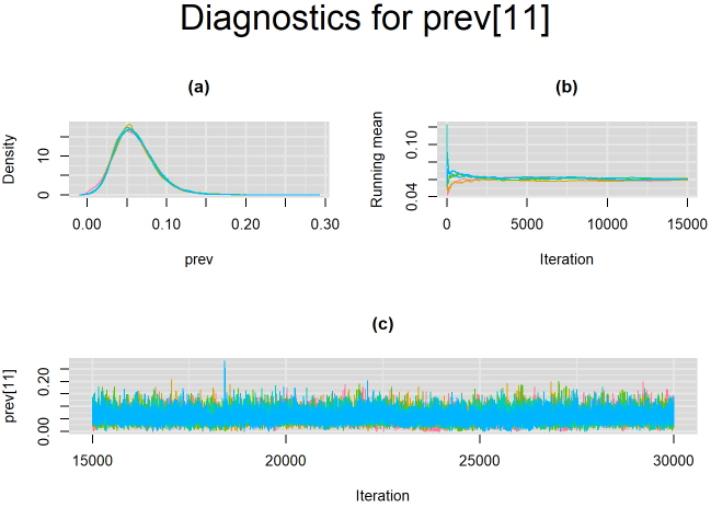
}For example, in the figure below, the posterior densities (a), running posterior mean values (b) and history plots (c) for the parameter prev[11] (prevalence of the 11th study) is displayed for each chain represented by different color. The very similar results from all five chains suggest the algorithm has converged to the same solution in each case.
SUMMARY STATISTICS
Once convergence of the MCMC algorithm is achieved, summary statistics of the parameters of interest may be extracted from their posterior distributions using the MCMCsummary function found in the MCMCvis package.
# Summary statistics
library(MCMCvis)
library(DT)
datatable(MCMCsummary(output, round=4), options = list(pageLength = 3) )
Below is the summary statistics output for the parameters shared across studies. The 50% quantile is the posterior median which is commonly used to estimate the paramater of interest. The 2.5% and 97.5% quantiles for the Predicted_Se and Predicted_Sp can be used to define prediction intervals for the mean sensitivity and mean specificity, respectively. If the prediction interval is much wider than the credible interval it would be indicative of high between-study heterogeneity in the index test.
The table also displays Rhat, which is the Gelman-Rubin statistic (Gelman and Ruben Gelman and Rubin (1992), Brooks and Gelman Brooks and Gelman (1998) ). It is enabled when 2 or more chains are generated. It evaluates MCMC convergence by comparing within- and between-chain variability for each model parameter. Rhat tends to 1 as convergence is approached.
Also, n.eff is the effective sample size (Gelman et al Gelman et al. (2013) ). Because the MCMC process causes the posterior draws to be correlated, the effective sample size is an estimate of the sample size required to achieve the same level of precision if that sample was a simple random sample. When draws are correlated, the effective sample size will generally be lower than the actual numbers of draws resulting in poor posterior estimates
SROC PLOT
The output from rjags can be used to obtain a plot in the summary receiver operating characteristic (SROC) space with 95% credible region (red line) and 95% prediction region (black dotted line) around the summary estimates of sensitivity and specificity (solid black circle) using the SROC_rjags function found in the DTAplots package. Individual studies can also be represented (blue circles) and are proportional to their sample size. The argument ref_std=FALSE is required to allow the plot to reflect the imperfect nature of the reference test.
# SROC plot
library(DTAplots)
SROC_rjags(X=output, model="Bivariate",n=n, study_col1="blue", study_col2=rgb(0, 0, 1, 0.15), dataset=cell, ref_std=FALSE, Sp.range=c(0.8,1))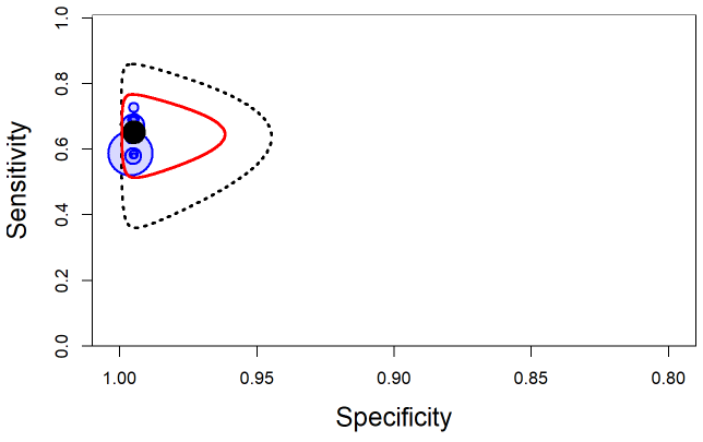
SCRIPT
For a copy of the complete script, please follow the link below
A PECULIARITY OF LATENT CLASS ANALYSIS
When using latent class analysis, it is not impossible the model may interchange the labels of target condition positive and target condition negative. This will usually result in different MCMC chains reaching apparently different but algebraically identical solutions, rendering the average results across chains probably not very meaningful. To illustrate this, we can run the same model (same seed value) that was run on the Xpert data presented earlier with non-informative priors but with less iterations. For instance, we will only run 15,000 burn-in iterations followed by 15,000 sampling iterations. But contrary to the model ran in the previous section where we had provided large initial value for mu2[2] in the first chain, here we will wrongly initialize that value to be -4 for all five chains, which translate into a 0.01799 value on the probability scale.
#Initial values
seed=37850
Listinits = list(
  GenInits(init_mu=c(0,0), init_mu2=c(0,-4), n=n),
  GenInits(init_mu=c(0,0), init_mu2=c(0,-4), n=n),
  GenInits(init_mu=c(0,0), init_mu2=c(0,-4), n=n),
  GenInits(init_mu=c(0,0), init_mu2=c(0,-4), n=n),
  GenInits(init_mu=c(0,0), init_mu2=c(0,-4), n=n))
The figure below monitors convergence of the parameter Summary_Sp2, which corresponds to the summary specificity of culture reference test. It shows that 4 of the 5 chains (chains 1, ,3, 4 and 5) converged to the same solution (posterior median around 0.98) while the 5th chain (chain number 2) seemed to converge to another solution (posterior median around 0.83 with more variability surrounding this estimate). Which of these solutions is the correct one?
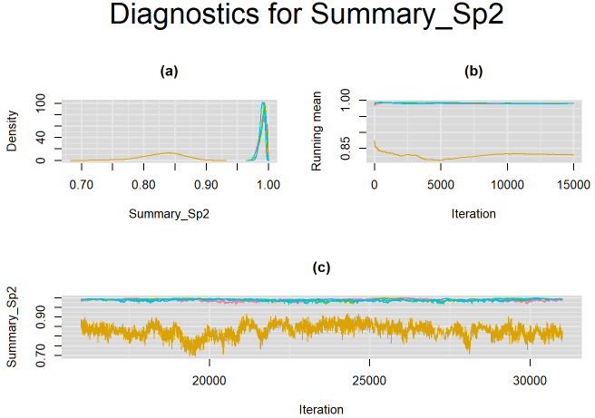
For this particular example, from prior experience it is known that culture has very high specificity. The solution attained by the 4 chains (posterior median around 0.98) is the correct one, while the solution attained by the lone chain (posterior median around 0.83) is not sensible.
A careful selection of initial values closer to the solution with the desired labelling will usually avoid the problem. Taking advantage of the knowledge we have on the high specificity of culture test, we provide initial values for the logit-transformed specificity of culture (mu2[2]) by assigning it a value of 4 which translate into a value of 0.98201 on the probability scale.
Listinits = list(
GenInits(init_mu=c(0,0), init_mu2=c(0,4), n=n),
GenInits(init_mu=c(0,0), init_mu2=c(0,4), n=n),
GenInits(init_mu=c(0,0), init_mu2=c(0,4), n=n),
GenInits(init_mu=c(0,0), init_mu2=c(0,4), n=n),
GenInits(init_mu=c(0,0), init_mu2=c(0,4), n=n)
)
# Compile the model
jagsModel = jags.model("model.txt",data=dataList,n.chains=5, n.adapt=0,inits=Listinits)
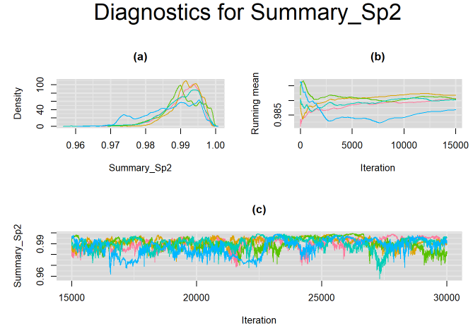
#jagsModel$state()This yields the following results, where all 5 chains are now converging closer to a single solution as depicted on the figure below. Can we improve the convergence?
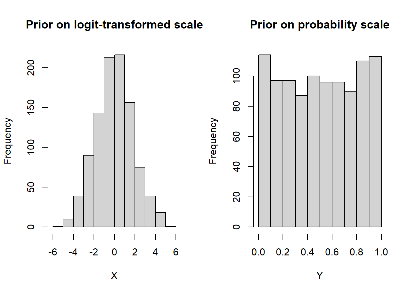
The rjags script described in the previous section comes with non-informative prior distributions. For instance, in the script, the logit-transformed mean sensitivity and specificity of both the index test and the reference test ( mu[1], mu[2], mu2[1] and mu2[2]) have a normal distribution with mean=0 and precision=0.3 as shown on the left-side panel of the figure below. When we transform this distribution on the probability scale, it tends to be uniformly distributed over the 0-1 range with the 2.5% and 97.5% quantiles approximately equal to 0.025 and 0.975 respectively.
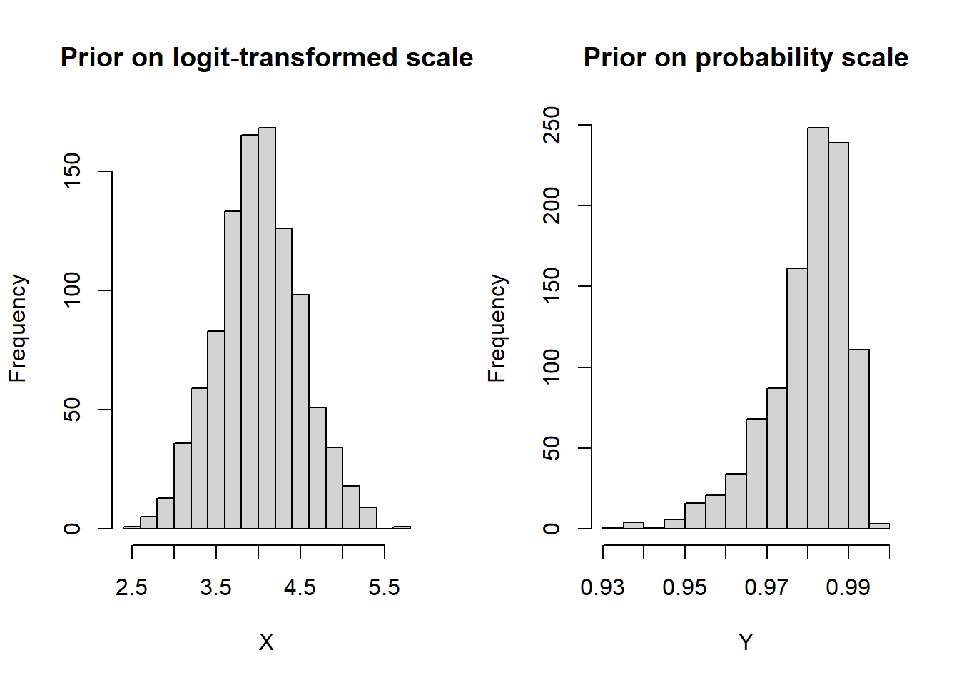
In some cases, redefining the prior distribution so that its domain only covers plausible values is helpful. Since it is believed that the culture (reference) test has a near perfect specificity, we incorporate this information in our model by specifying an informative prior distribution for the parameter mu2[2]. A normal distribution with mean=4 and precision=4 is placed on mu2[2]. This prior distribution places much of its weight on probability values that are greater than 0.95 (see right-side panel of figure below)
To demonstrate this, we are going to initialize the chains with the bad initial values used above.
#Initial values
seed=37850
Listinits = list(
  GenInits(init_mu=c(0,0), init_mu2=c(0,-4), n=n),
  GenInits(init_mu=c(0,0), init_mu2=c(0,-4), n=n),
  GenInits(init_mu=c(0,0), init_mu2=c(0,-4), n=n),
  GenInits(init_mu=c(0,0), init_mu2=c(0,-4), n=n),
  GenInits(init_mu=c(0,0), init_mu2=c(0,-4), n=n))
After running the model with the informative prior on culture test’s specificity, with 15,000 burn-in iterations and 15,000 sampling iterations, all 5 chains are now satisfyingly converging to the same solution, as we can see in the figure below.

Below is a copy of the complete script to run the Bayesian Bivariate latent class meta-analysis model in rjags. The script uses the model with informative prior on specificity of culture reference test.
####################################
#### DATA FOR MOTIVATING EXAMPLE ###
####################################
t11 <- c(7, 6, 2, 5, 0, 1, 4, 3, 3, 1, 7, 35, 103, 1, 2, 22, 6, 25, 27, 15, 5, 2, 2, 11, 2, 0, 8, 3, 1)
t10 <- c(5, 4, 0, 0, 0, 0, 6, 0, 3, 0, 0, 5, 6, 1, 0, 1, 1, 3, 11, 3, 9, 3, 0, 2, 4, 0, 2, 0, 2)
t01 <- c(5, 4, 0, 1, 2, 0, 8, 1, 1, 0, 0, 1, 18, 2, 0, 5, 0, 20, 25, 7, 10, 1, 1, 2, 2, 3, 5, 0, 0)
t00 <- c(63, 115, 2, 44, 132, 4, 83, 250, 67, 14, 150, 119, 252, 107, 8, 31, 148, 687, 204, 205, 115, 53, 4, 118, 22, 16, 186, 28, 43)
cell <- cbind(t11, t10, t01, t00)
n <- length(t11)  #  Number of studies
n.study <- rowSums(cell) #  Study sample sizes
dataList <- list(t12=cell,n=n, n.study=n.study)

#################
### THE MODEL ###
#################
modelString =
  "model {

#=== LIKELIHOOD ===#
for(i in 1:n) {

t12[i,1:4] ~ dmulti(p12[i,1:4],n.study[i])

p12[i,1] <- prev[i]*( se[i]* se2[i]     +covp[i]) + (1-prev[i])*( (1-sp[i])*(1-sp2[i]) +covn[i])
p12[i,2] <- prev[i]*( se[i]* (1-se2[i]) -covp[i]) + (1-prev[i])*( (1-sp[i])*sp2[i]     -covn[i])
p12[i,3] <- prev[i]*( (1-se[i])*se2[i]     -covp[i]) + (1-prev[i])*( sp[i]*(1-sp2[i]) -covn[i])
p12[i,4] <- prev[i]*( (1-se[i])*(1-se2[i]) +covp[i]) + (1-prev[i])*( sp[i]*sp2[i] +covn[i])


# Hierarchical prior distribution for XPERT test
logit(se[i]) <- l[i,1]
logit(sp[i]) <- l[i,2]
l[i,1:2] ~ dmnorm(mu[1:2], T[1:2,1:2])

# Hierarchical prior distribution for CUTURE test
logit(se2[i]) <- l2[i,1]
logit(sp2[i]) <- l2[i,2]
l2[i,1:2] ~ dmnorm(mu2[1:2],T2[1:2,1:2])

# Prior distribution for prevalence
prev[i] ~ dbeta(1,1)

#=== CONDITIONAL DEPENDENCE STRUCTURE ===#
# lower and upper limits of covariance parameters
maxs12[i]<-min(se[i],se2[i])-(se[i]*se2[i])
maxc12[i]<-min(sp[i],sp2[i])-(sp[i]*sp2[i])
mins12[i]<- (1-se[i])*(se2[i]-1)
minc12[i]<- (1-sp[i])*(sp2[i]-1)

# covariance parameters
covp[i] ~ dunif(mins12[i], maxs12[i]);
covn[i] ~ dunif(minc12[i], maxc12[i]);
}

####    HYPER PRIOR DISTRIBUTIONS FOR XPERT ACCURACY    ####
# prior for the logit transformed sensitivity (mu[1]) and logit transformed  specificity (mu[2]) of XPERT test
mu[1] ~ dnorm(0,0.3)
mu[2] ~ dnorm(0,0.3)

# Between-study variance-covariance matrix of XPERT test
T[1:2,1:2]<-inverse(TAU[1:2,1:2])
TAU[1,1] <- tau[1]*tau[1]
TAU[2,2] <- tau[2]*tau[2]
TAU[1,2] <- rho*tau[1]*tau[2]
TAU[2,1] <- rho*tau[1]*tau[2]

# prior for the between-study precision of the logit transformed sensitivity (prec[1]) and logit transformed specificity (prec[2]) of XPERT test
prec[1] ~ dgamma(2,0.5)
prec[2] ~ dgamma(2,0.5)
rho ~ dunif(-1,1)

####    HYPER PRIOR DISTRIBUTIONS FOR CULTURE ACCURACY    ####
# prior for the logit transformed sensitivity (mu[1]) and logit transformed  specificity (mu[2]) of CULTURE test
mu2[1] ~ dnorm(0,0.3)
mu2[2] ~ dnorm(4,4)

# Between-study variance-covariance matrix of CULTURE test
T2[1:2,1:2] <- inverse(TAU2[1:2,1:2])
TAU2[1,1] <- tau2[1]*tau2[1]
TAU2[2,2] <- tau2[2]*tau2[2]
TAU2[1,2] <- rho2*tau2[1]*tau2[2]
TAU2[2,1] <- rho2*tau2[1]*tau2[2]

# prior for the between-study precision of the logit transformed sensitivity (prec2[1]) and logit transformed specificity (prec2[2]) of CULTURE test
prec2[1] ~ dgamma(2,0.5)
prec2[2] ~ dgamma(2,0.5)
rho2 ~ dunif(-1,1)

####  OTHER PARAMETERS OF INTEREST

# Between-study standard deviation of the logit transformed sensitivity (tau[1]) and specificity (tau[2]) of XPERT test
tau[1]<-pow(prec[1],-0.5)
tau[2]<-pow(prec[2],-0.5)
tau.sq[1]<-pow(prec[1],-1)
tau.sq[2]<-pow(prec[2],-1)

# Between-study standard deviation of the logit transformed sensitivity (tau2[1]) and specificity (tau2[2]) of CULTURE test
tau2[1] <- pow(prec2[1],-0.5)
tau2[2] <- pow(prec2[2],-0.5)

# Mean sensitivity and mean specificity of XPERT
Summary_Se <-1/(1+exp(-mu[1]))
Summary_Sp <-1/(1+exp(-mu[2]))

# Predicted sensitivity and predicted specificity of XPERT in a future study
l.predict[1:2] ~ dmnorm(mu[],T[,])
Predicted_Se <- 1/(1+exp(-l.predict[1]))
Predicted_Sp <- 1/(1+exp(-l.predict[2]))

# Mean sensitivity and mean specificity of CULTURE
Summary_Se2<-1/(1+exp(-mu2[1]))
Summary_Sp2<-1/(1+exp(-mu2[2]))

# Predicted sensitivity and predicted specificity of CULTURE in a future study
l.predict2[1:2] ~ dmnorm(mu2[],T2[,])
Predicted.Se2 <- 1/(1+exp(-l.predict2[1]))
Predicted.Sp2 <- 1/(1+exp(-l.predict2[2]))
}"

writeLines(modelString,con="model_inform_prior.txt")

######################
### INITIAL VALUES ###
######################
GenInits = function(init_mu=NULL, init_mu2=NULL, Seed=seed, n){
  if(is.null(init_mu) == FALSE & is.null(init_mu2) == FALSE){
    mu = c(as.numeric(init_mu[1]),as.numeric(init_mu[2]))
    mu2 = c(as.numeric(init_mu2[1]),as.numeric(init_mu2[2]))
  }
  else{
    mu=c(rnorm(1,0,1/sqrt(0.3)),rnorm(1,0,1/sqrt(0.3)))
    mu2=c(rnorm(1,0,1/sqrt(0.3)),rnorm(1,4,1/sqrt(4)))
  }
  list(
    mu=mu,
    mu2=mu2,
    covn = rep(0,n),
    covp = rep(0,n),
    prev = runif(n),
    prec = c(rgamma(1,2,0.5),rgamma(1,2,0.5)),
    prec2 = c(rgamma(1,2,0.5),rgamma(1,2,0.5)),
    rho = runif(1,-1,1),
    rho2 = runif(1,-1,1) ,
    .RNG.name="base::Wichmann-Hill",
    .RNG.seed=Seed
  )
}
seed=24050; set.seed(seed)
Listinits = list(
  GenInits(n=n),
  GenInits(n=n),
  GenInits(n=n),
  GenInits(n=n),
  GenInits(n=n)
)

#######################################
### COMPILING AND RUNNING THE MODEL ###
#######################################
library(rjags)
jagsModel = jags.model("model.txt",data=dataList,n.chains=5,inits=Listinits,n.adapt=0)
# Burn-in iterations
update(jagsModel,n.iter=30000)
# Parameters to be monitored
parameters = c( "prev", "se","sp", "se2", "sp2", "mu", "mu2",  "tau", "tau2", "rho", "rho2", "Summary_Se", "Summary_Se2", "Summary_Sp", "Summary_Sp2", "Predicted_Se", "Predicted_Sp")
# Posterior samples
output = coda.samples(jagsModel,variable.names=parameters,n.iter=30000)
##############################
### MONITORING CONVERGENCE ###
##############################
library(mcmcplots)
# Plots to check convergence for parameters varying across studies:
# Index j refers to the number of studies
# Index n refers to the number of studies
# Index i follows the ordering of the parameters vector defined above.  If left unchanged :
# i = 1 : disease prevalence in study j (prev)
# i = 2 : sensitivity in study j (se)
# i = 3 : specificity in study j (sp)
# i = 4 : sensitivity in study j (se2)
# i = 5 : specificity in study j (sp2)

for(j in 1:n) {
for(i in c(1:5)) {
  #  tiff(paste(parameters[i],"[",j,"] Converged",".tiff",sep=""),width = 23, height = 23, units = "cm", res=200)
  par(oma=c(0,0,3,0))
  layout(matrix(c(1,2,3,3), 2, 2, byrow = TRUE))
  denplot(output, parms=c(paste(parameters[i],"[",j,"]",sep="")), auto.layout=FALSE, main="(a)", xlab=paste(parameters[i],"",sep=""), ylab="Density")
  rmeanplot(output, parms=c(paste(parameters[i],"[",j,"]",sep="")), auto.layout=FALSE, main="(b)")
  title(xlab="Iteration", ylab="Running mean")
  traplot(output, parms=c(paste(parameters[i],"[",j,"]",sep="")), auto.layout=FALSE, main="(c)")
  title(xlab="Iteration", ylab=paste(parameters[i],"[",j,"]",sep=""))
  mtext(paste("Diagnostics for ", parameters[i],"[",j,"]","",sep=""), side=3, line=1, outer=TRUE, cex=2)
  #  dev.off()
}
}
# Plots to check convergence for parameters shared across studies:
# Index j = 1 refers to sensitivity and j = 2 refers to specificity
# Index i follows the ordering of the parameters vector defined above.  If left unchanged :
# i = 6 : logit-transformed mean sensitivity of index test (j=1) and logit-transformed mean specificity of index test (j=2) (mu)
# i = 7 : logit-transformed mean sensitivity of reference test (j=1) and logit-transformed mean specificity of reference test (j=2) (mu2)
# i = 8 : between-study standard deviation in logit-transformed sensitivity of index test (j=1) and between-study standard deviation in logit-transformed specificity of index test (j=2) (tau)
# i = 9 : between-study standard deviation in logit-transformed sensitivity of reference test (j=1) and between-study standard deviation in logit-transformed specificity of reference test (j=2) (tau2)
for(j in 1:2) {
for(i in c(6:9)) {
#  tiff(paste(parameters[i],"[",j,"] Converged",".tiff",sep=""),width = 23, height = 23, units = "cm", res=200)
  par(oma=c(0,0,3,0))
  layout(matrix(c(1,2,3,3), 2, 2, byrow = TRUE))
  denplot(output, parms=c(paste(parameters[i],"[",j,"]",sep="")), auto.layout=FALSE, main="(a)", xlab=paste(parameters[i],"",sep=""), ylab="Density")
  rmeanplot(output, parms=c(paste(parameters[i],"[",j,"]",sep="")), auto.layout=FALSE, main="(b)")
  title(xlab="Iteration", ylab="Running mean")
  traplot(output, parms=c(paste(parameters[i],"[",j,"]",sep="")), auto.layout=FALSE, main="(c)")
  title(xlab="Iteration", ylab=paste(parameters[i],"[",j,"]",sep=""))
  mtext(paste("Diagnostics for ", parameters[i],"[",j,"]","",sep=""), side=3, line=1, outer=TRUE, cex=2)
#  dev.off()
}
}

# Index j not needed for the following shared parameters
# i = 10 : correlation between logit-transformed sensitivity of index test and logit-transformed specificity of index test (rho)
# i = 11 : correlation between logit-transformed sensitivity of reference test and logit-transformed specificity of reference test (rho2)
# i = 12: mean sensitivity of index test (Summary_Se)
# i = 13: mean sensitivity of reference test (Summary_Se2)
# i = 14: mean specificity of index test (Summary_Sp)
# i = 15: mean specificity of reference test (Summary_Sp2)
# i = 16: predicted sensitivity of index test in a future study (Predicted_Se)
# i = 17: predicted specificity of index test in a future study (Predicted_Sp)


for(i in 10:17) {
#  tiff(paste(parameters[i]," Converged",".tiff",sep=""),width = 23, height = 23, units = "cm", res=200)
  par(oma=c(0,0,3,0))
  layout(matrix(c(1,2,3,3), 2, 2, byrow = TRUE))
  denplot(output, parms=c(paste(parameters[i], sep="")), auto.layout=FALSE, main="(a)", xlab=paste(parameters[i],"",sep=""), ylab="Density")
  rmeanplot(output, parms=c(paste(parameters[i], sep="")), auto.layout=FALSE, main="(b)")
  title(xlab="Iteration", ylab="Running mean")
  traplot(output, parms=c(paste(parameters[i], sep="")), auto.layout=FALSE, main="(c)")
  title(xlab="Iteration", ylab=paste(parameters[i], sep=""))
  mtext(paste("Diagnostics for ", parameters[i], sep=""), side=3, line=1, outer=TRUE, cex=2)
#  dev.off()
}

##########################
### SUMMARY STATISTICS ###
##########################
library(MCMCvis)
library(DT)
datatable(MCMCsummary(output, round=4), options = list(pageLength = 3) )

#################
### SROC PLOT ###
#################
library(DTAplots)
SROC_rjags(X=output, model="Bivariate",n=n, study_col1="blue", study_col2=rgb(0, 0, 1, 0.15), dataset=cell, ref_std=FALSE, Sp.range=c(0.8,1))
REFERENCES
Citation
@online{schiller2021,
  author = {Ian Schiller and Nandini Dendukuri},
  title = {Bayesian Inference for the {Bivariate} Latent Class Model for
    Diagnostic Meta-Analysis},
  date = {2021-04-20},
  url = {https://www.nandinidendukuri.com/blogposts/2021-04-20-bayesian-LC-meta-analysis/},
  langid = {en}
}