Bayesian Bivariate Model
Saliva_COVID DATASET
The Saliva_COVID database includes 6013 participants spread across 17 studies as follow. The Saliva_COVID data is from Butler-Laporte et al(2021)
BAYESIAN BIVARIATE META-ANALYSIS MODEL SPECIFICATION
# Bayesian bivariate model
modelString =

"model {
#=== LIKELIHOOD ===#
for(i in 1:n) {
TP[i] ~ dbin(se[i],pos[i])
TN[i] ~ dbin(sp[i],neg[i])

# === PRIOR FOR INDIVIDUAL LOGIT SENSITIVITY AND SPECIFICITY === #
logit(se[i]) <- l[i,1]
logit(sp[i]) <- l[i,2]
l[i,1:2] ~ dmnorm(mu[], T[,])
}

#=== HYPER PRIOR DISTRIBUTIONS POOLED LOGIT SENSITIVITY AND SPECIFICITY === #
mu[1] ~ dnorm(0,0.25)
mu[2] ~ dnorm(0,0.25)
# Between-study variance-covariance matrix

T[1:2,1:2]<-inverse(TAU[1:2,1:2])
TAU[1,1] <- tau[1]*tau[1]
TAU[2,2] <- tau[2]*tau[2]
TAU[1,2] <- rho*tau[1]*tau[2]
TAU[2,1] <- rho*tau[1]*tau[2]
#=== HYPER PRIOR DISTRIBUTIONS FOR PRECISION OF LOGIT SENSITIVITY ===#
#=== AND LOGIT SPECIFICITY, AND CORRELATION BETWEEN THEM === #
prec[1] ~ dgamma(2,0.5)
prec[2] ~ dgamma(2,0.5)
rho ~ dunif(-1,1)

# ===  PARAMETERS OF INTEREST === #
# BETWEEN-STUDY STANDARD DEVIATION (tau) AND VARIANCE (tau.sq) OF LOGIT SENSITIVITY AND SPECIFICITY
tau[1]<-pow(prec[1],-0.5)
tau[2]<-pow(prec[2],-0.5)
tau.sq[1]<-pow(prec[1],-1)
tau.sq[2]<-pow(prec[2],-1)
# SUMMARY SENSITIVITY AND SPECIFICITY
Summary_Se <- 1/(1+exp(-mu[1]))
Summary_Sp <- 1/(1+exp(-mu[2]))
# PREDICTED SENSITIVITY AND SPECIFICITY IN A NEW STUDY
l.predicted[1:2] ~ dmnorm(mu[],T[,])
Predicted_Se <- 1/(1+exp(-l.predicted[1]))
Predicted_Sp <- 1/(1+exp(-l.predicted[2]))
}
"
The posterior samples were obtained by running the bivariate model (Reitsma et al(2005)) with 3 independent chains each having their own starting values to assess convergence of the MCMC algorithm. For each chain, after discarding the first 100 iterations (burn-in), we kept the next 100 iterations to form a posterior samples of 300 iterations.
This model uses prior distributions on the log-odds scale over the pooled sensitivity and specificity parameters (normal distribution with mean 0 and a variance of 4), their corresponding between-study precision on the log odds scale (gamma distribution with a shape parameter of 2 and a rate parameter of 0.5), and the correlation terms (uniform distribution whose upper and lower limits are -1 and 1, respectively). The precision is defined as the reciprocal of the variance.
POSTERIOR RESULTS
Posterior mean, standard deviation (sd) as well as posterior median (50%) and the 95% credible interval (2.5% and 97.5%) statistics are presented below. Convergence statistics are also provided.
Rhatis the Gelman-Rubin statistic (Gelman and Ruben(1992), Brooks and Gelman(1998)). It is enabled when 2 or more chains are generated. It evaluates MCMC convergence by comparing within- and between-chain variability for each model parameter.Rhattends to 1 as convergence is approached.n.effis the effective sample size (Gelman et al(2013)). Because the MCMC process causes the posterior draws to be correlated, the effective sample size is an estimate of the sample size required to achieve the same level of precision if that sample was a simple random sample. When draws are correlated, the effective sample size will generally be lower than the actual numbers of draws resulting in poor posterior estimates.
Posterior estimates are provided for the following parameters :
- Predicted sensitivity in a future sutdy, noted as Predicted_Se
- Predicted specificity in a future study, noted as Predicted_Sp
- Summary sensitivity across all studies, noted as Summary_Se
- Summary specificity across all studies, noted as Summary_Sp
- Mean logit-transformed sensitivity, noted as mu[1]
- Mean logit-transformed sensitivity, noted as mu[2]
- Correlation between the mean logit-transformed sensitivity and the mean logit-transformed specificity, noted as rho
- Sensitivity in individual studies, noted as se[i], where i is the study identifier
- Specificity in individual studies, noted as sp[i], where i is the study identifier
- Between-study standard deviation in the logit-transformed sensitivity, noted as tau[1]
- Between-study standard deviation in the logit-transformed specificity, noted as tau[2]
- Between-study variance in the logit-transformed sensitivity, noted as tau.sq[1]
- Between-study variance in the logit-transformed specificity, noted as tau.sq[2]
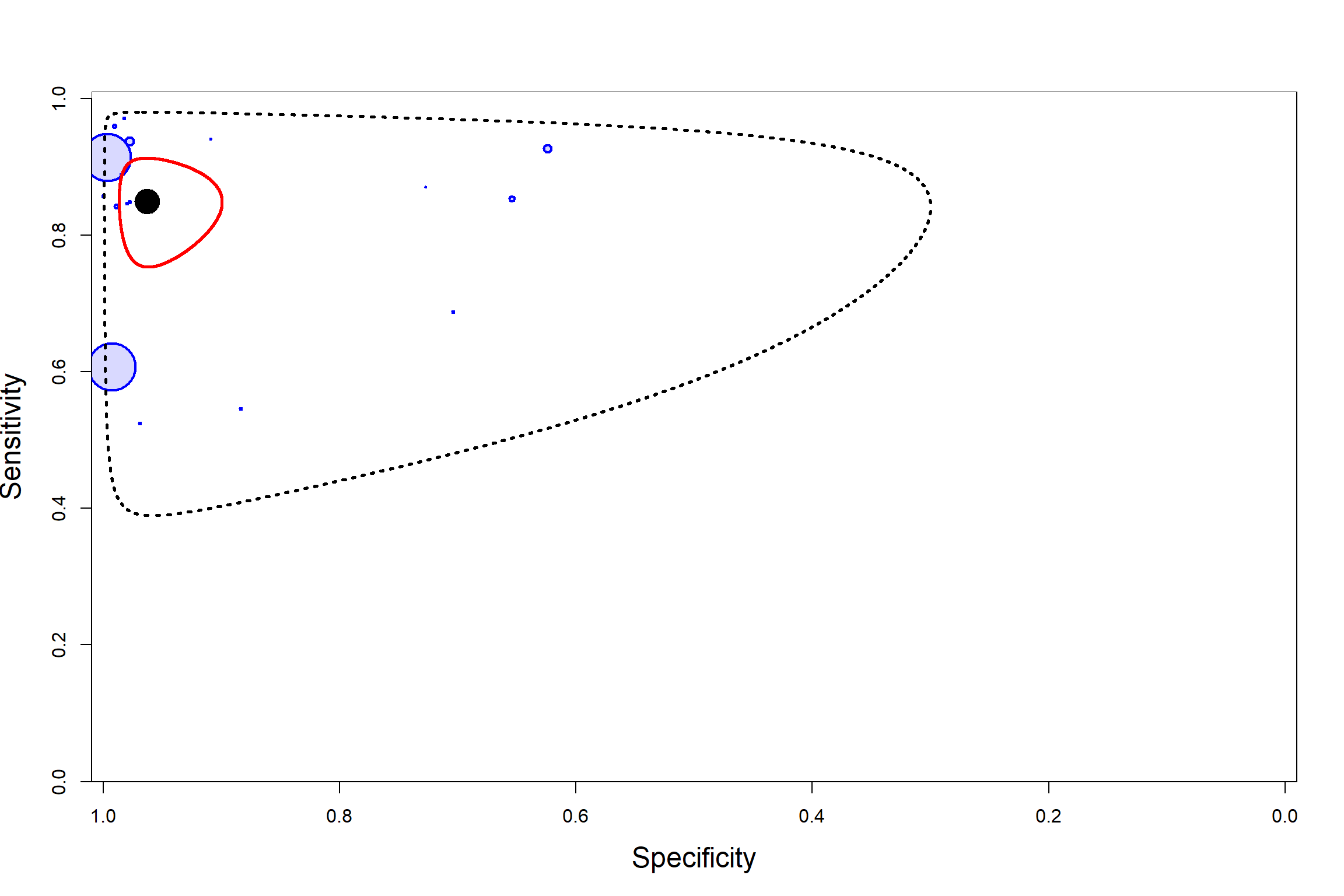
POSTERIOR ESTIMATES NEEDED TO CREATE SROC PLOT IN RevMan
The following posterior estimates are required in order to create the SROC plot in RevMan :
- E(logitSe) : Mean logit-transformed sensitivity, mu[1] = 1.7332
- E(logitSp) : Mean logit-transformed sensitivity, mu[2] = 3.2384
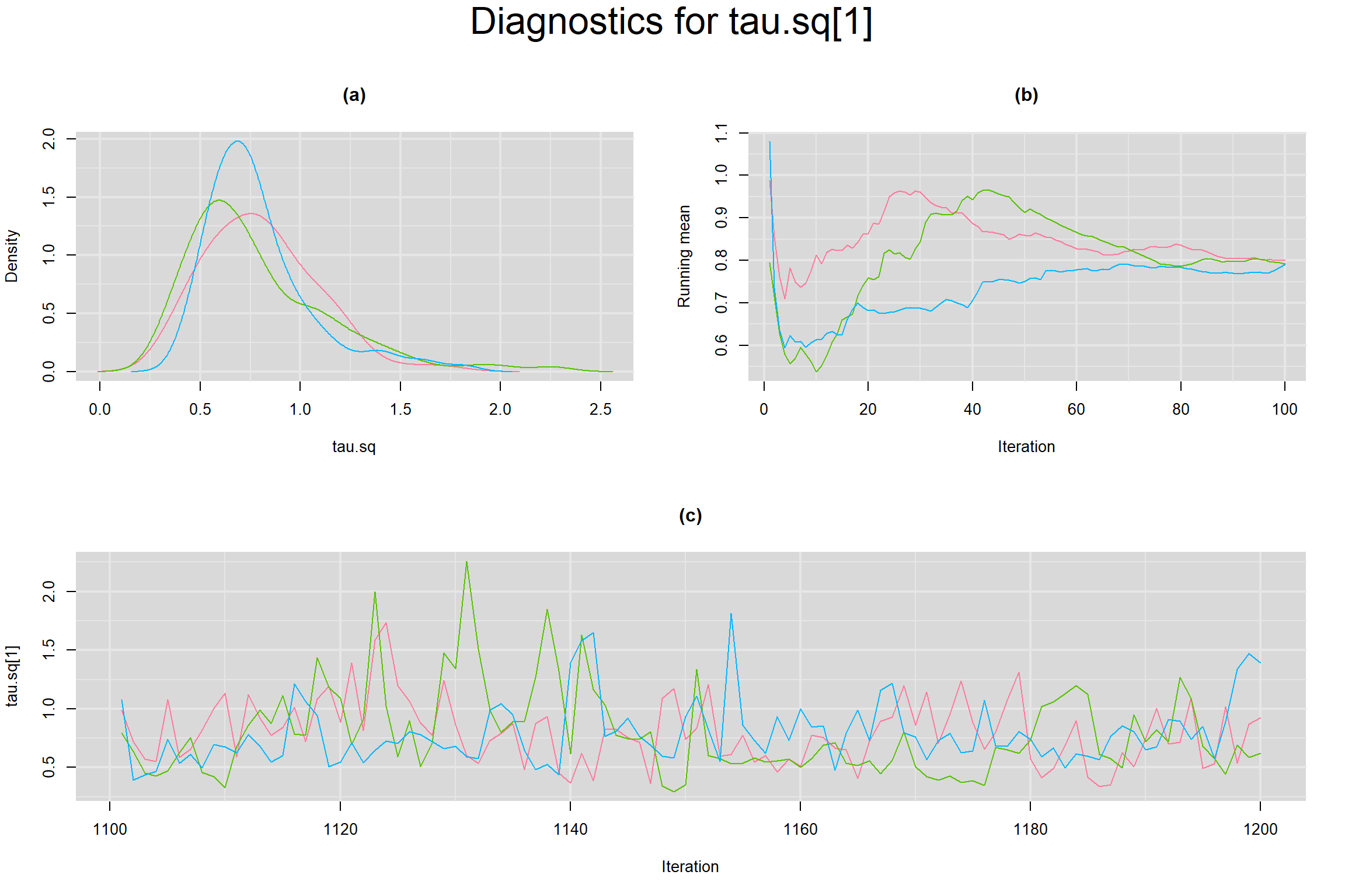
- Var(logitSe) : Between-study variance in the logit-transformed sensitivity, tau.sq[1] = 0.7949
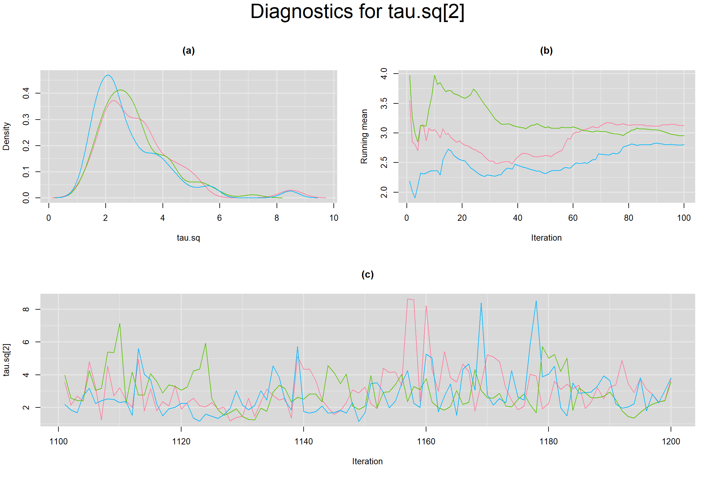
- Var(logitSp) : Between-study variance in the logit-transformed specificity, tau.sq[2] = 2.9663
- Corr(logits) : Correlation between the mean logit-transformed sensitivity and the mean logit-transformed specificity, rho = 0.073
- Cov(Es) : Covariance between the posterior samples of the mean logit-transformed sensitivity and mean logit-transformed specificity, 0.0018
- SE(E(logitSe)) : Estimated standard error of mean logit-transformed sensitivity = 0.2518
- SE(E(logitSp)) : Estimated standard error of mean logit-transformed specificity = 0.4338
SUMMARY ROC PLOT
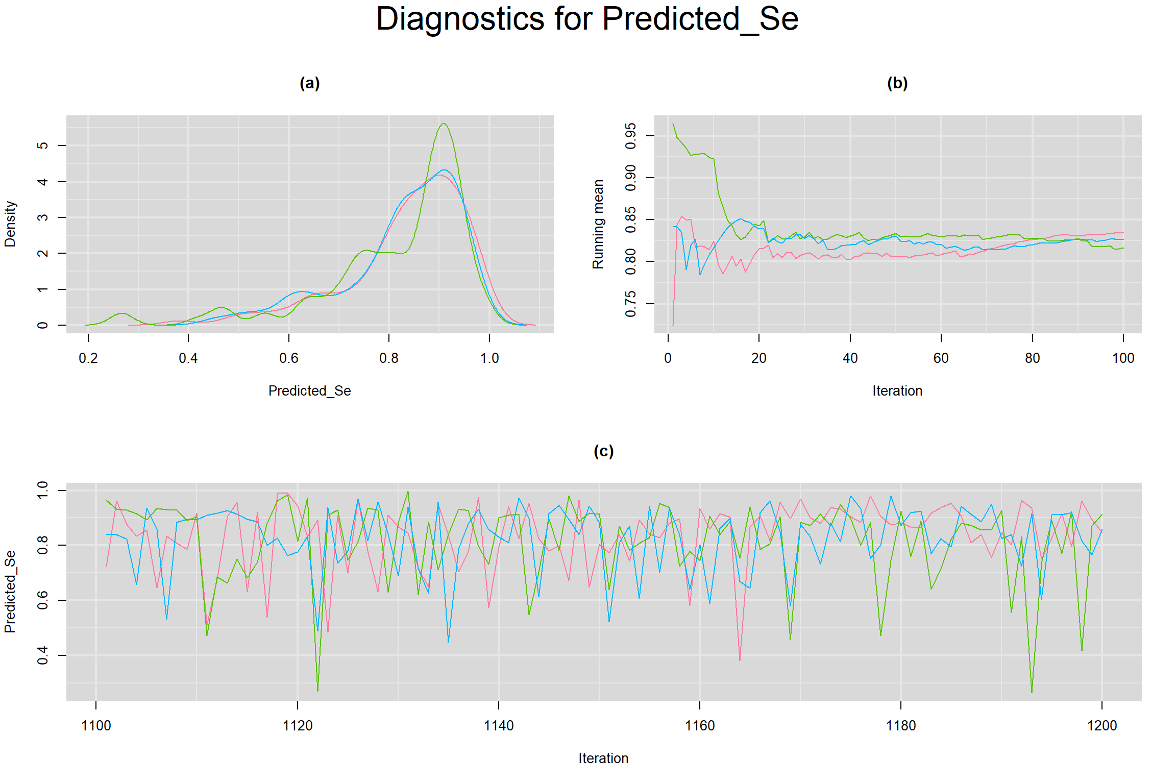
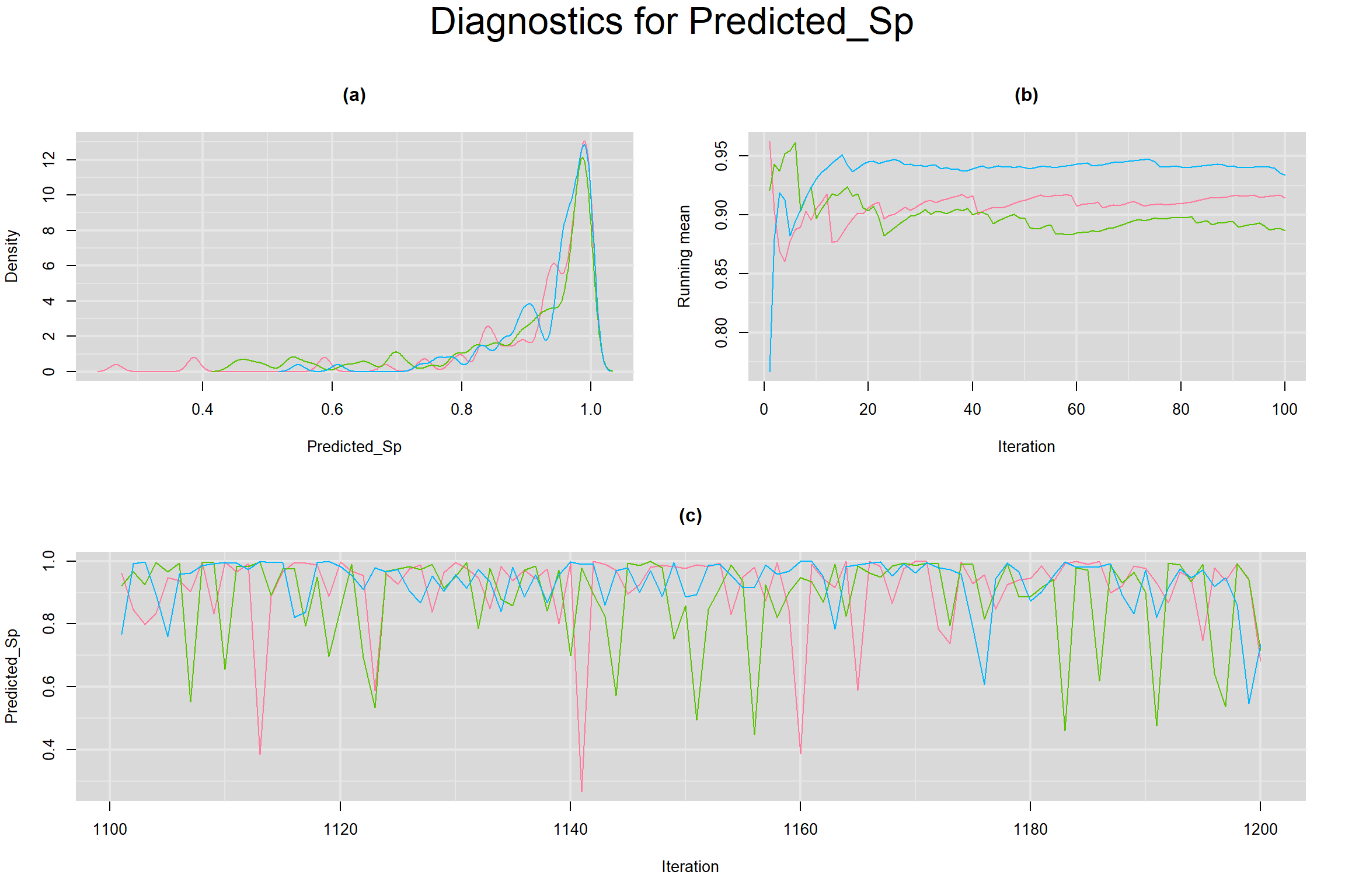
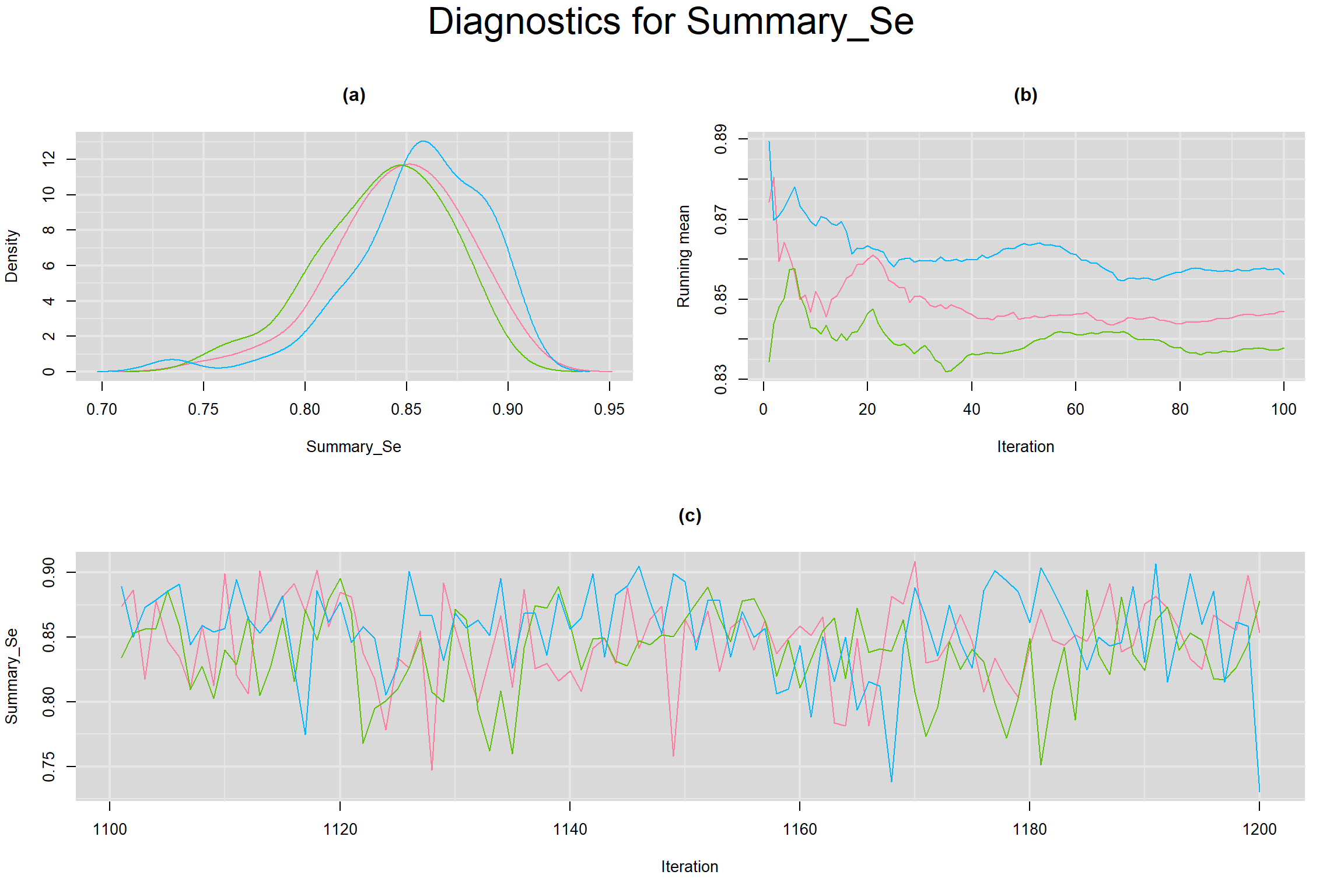
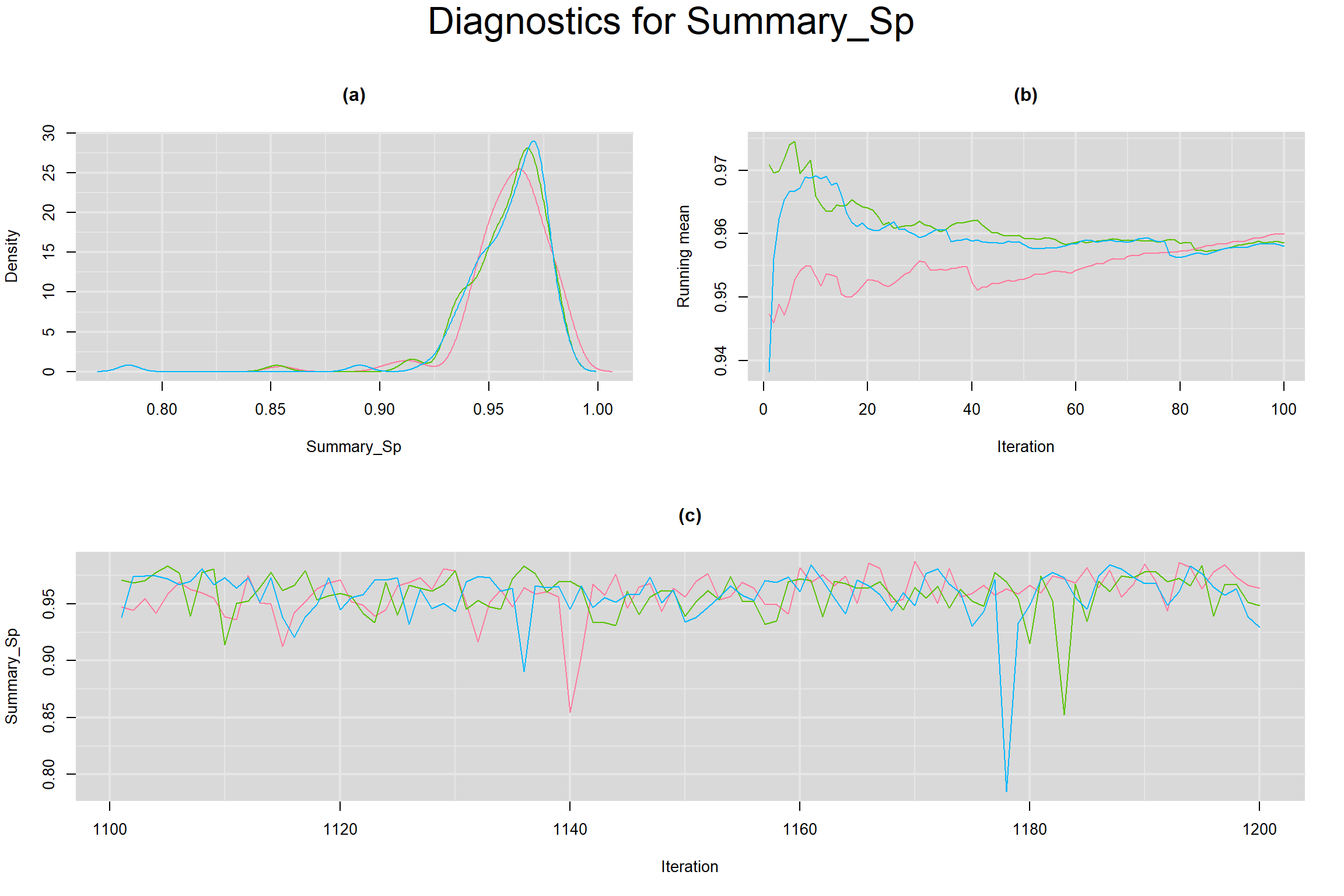
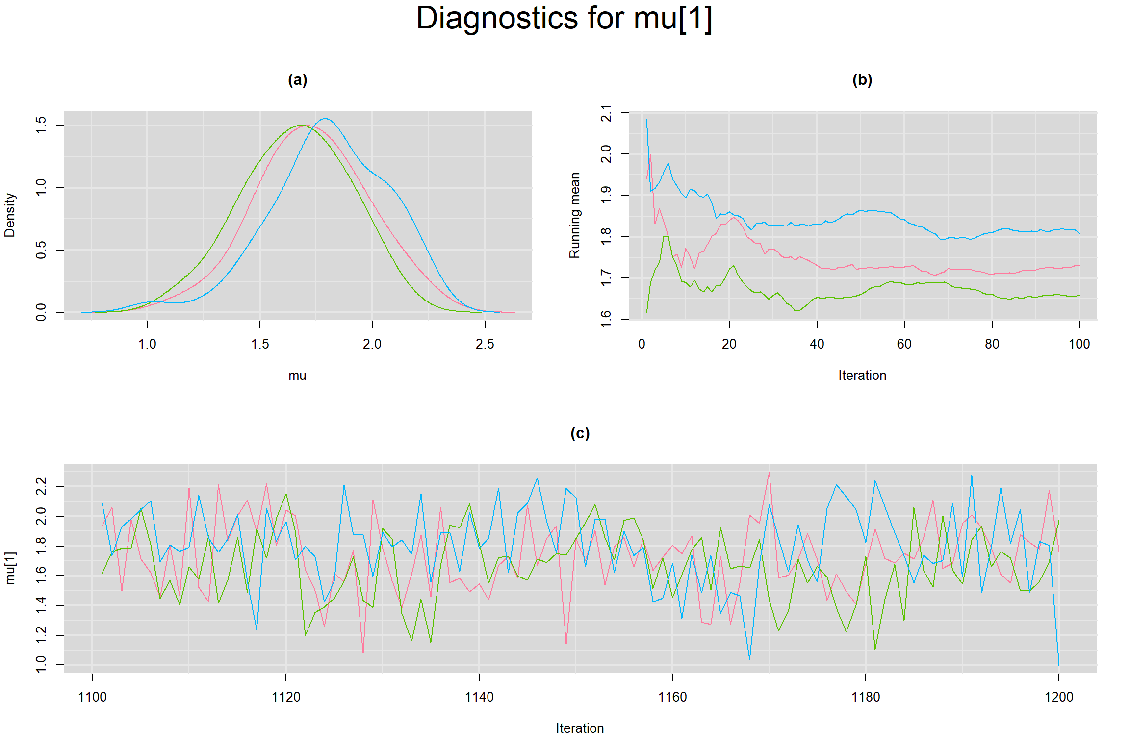
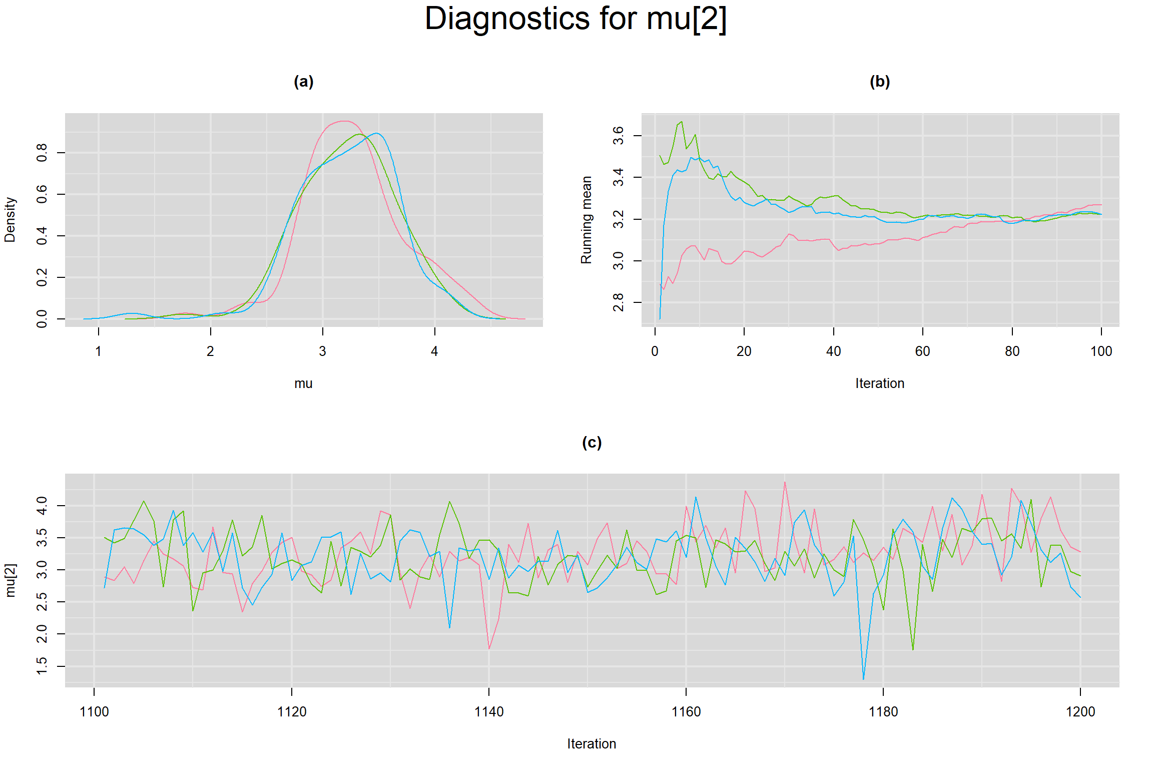
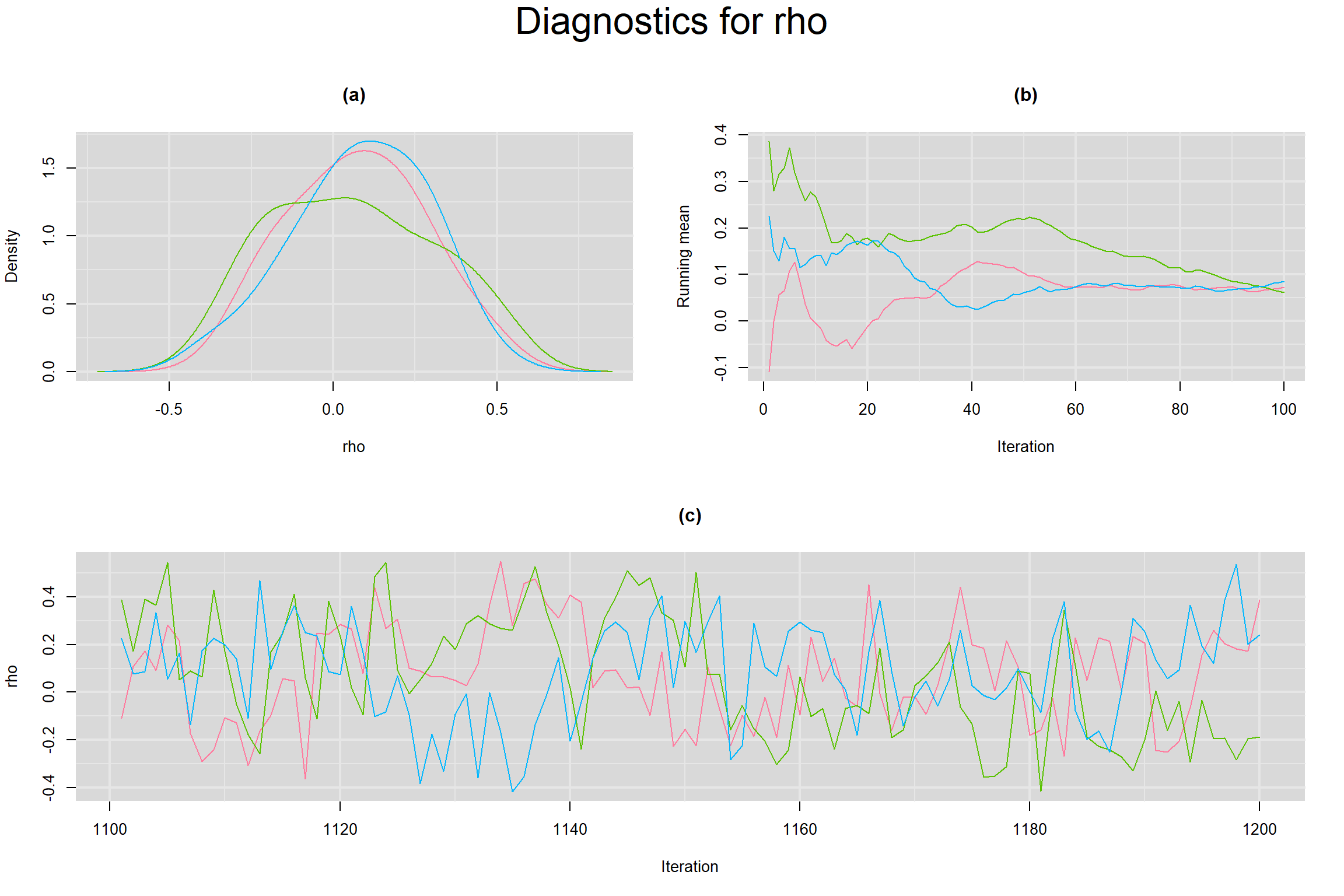
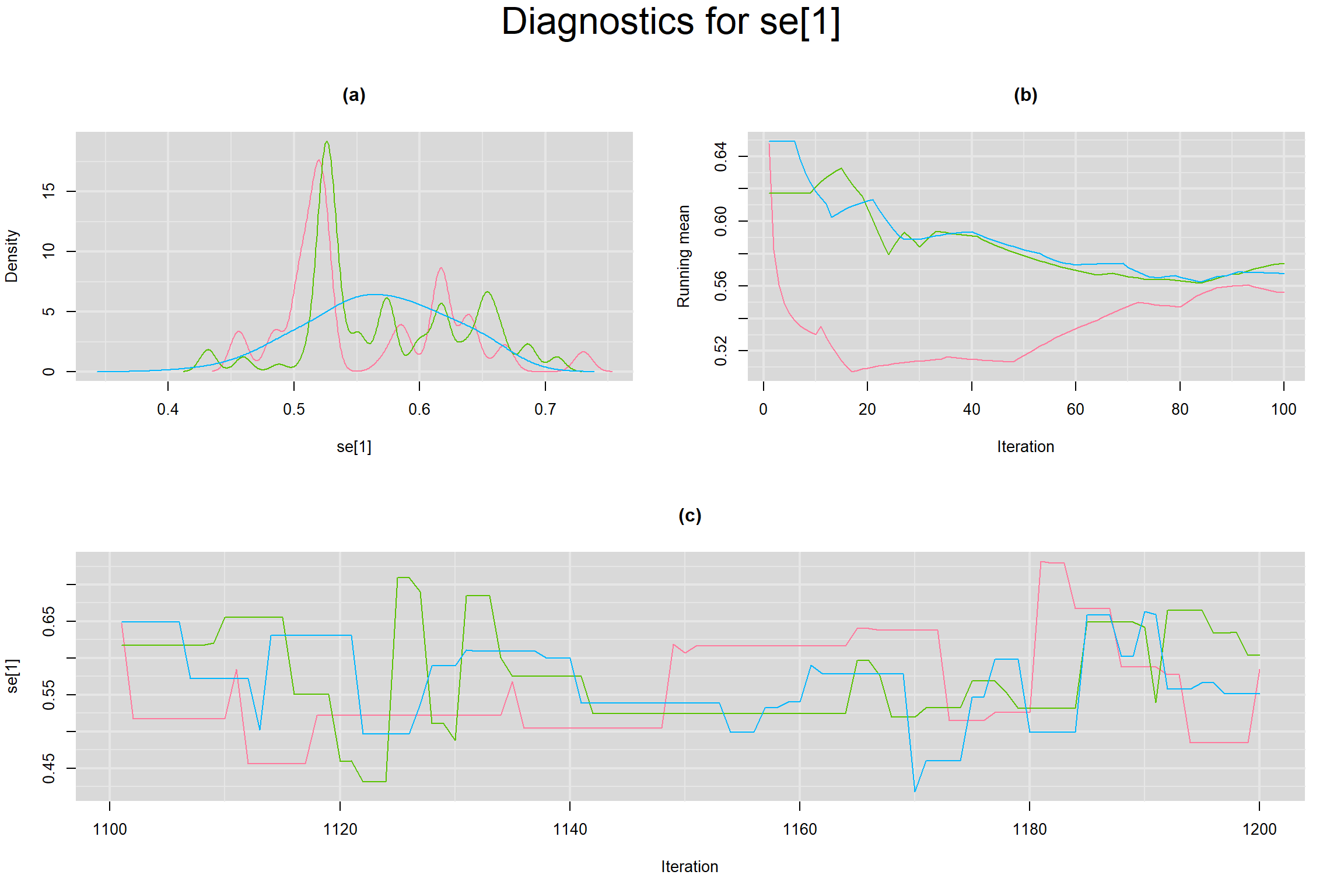
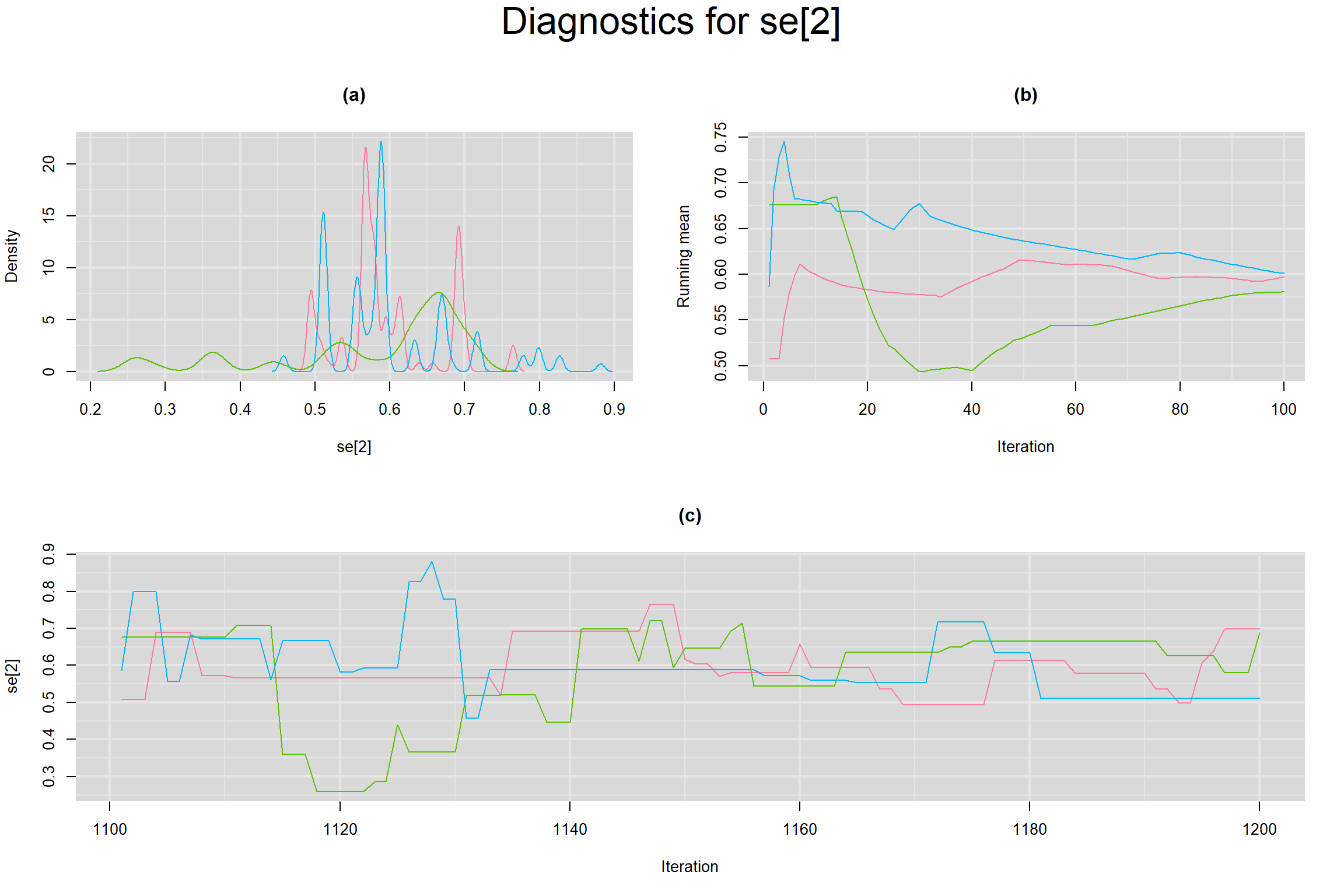
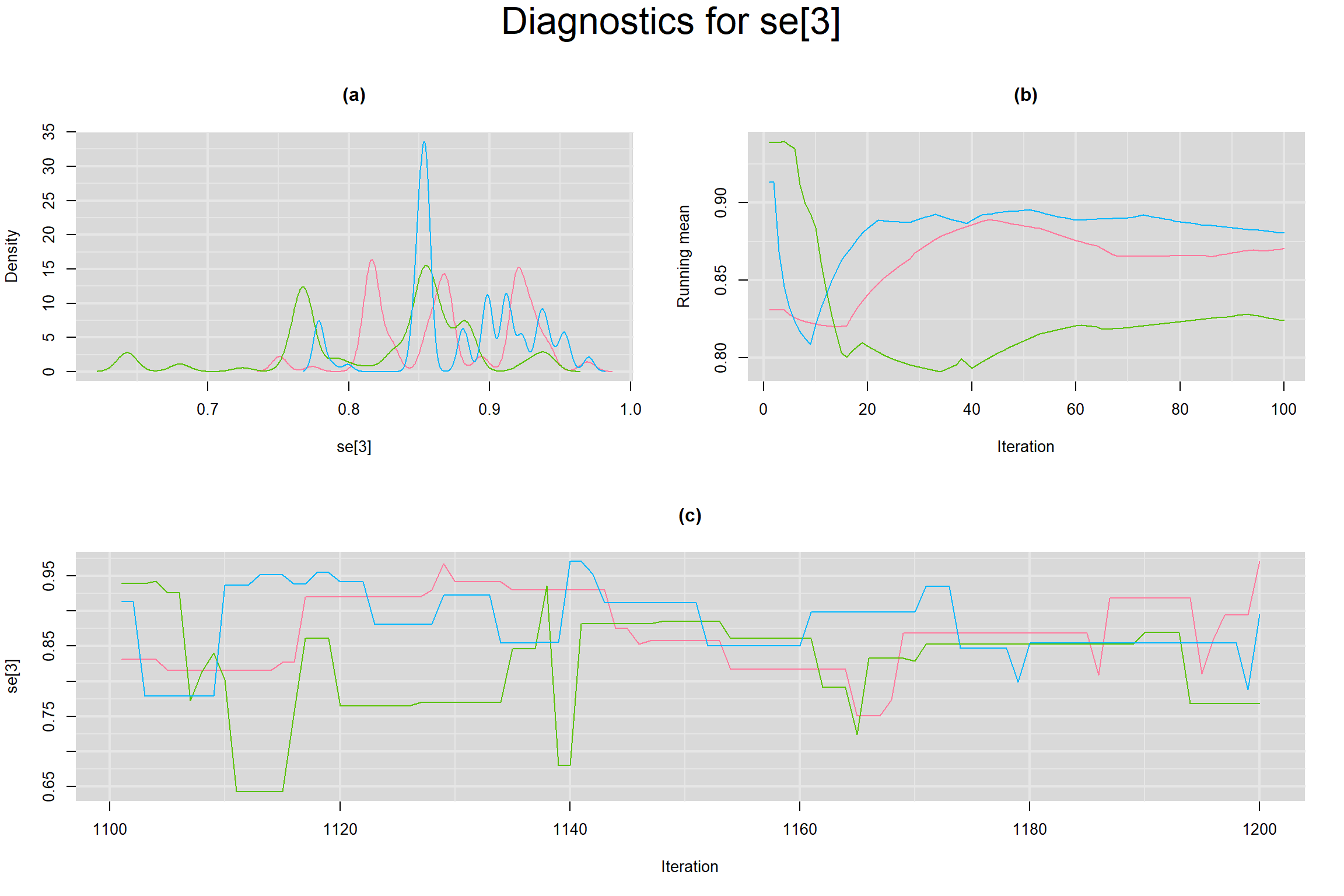
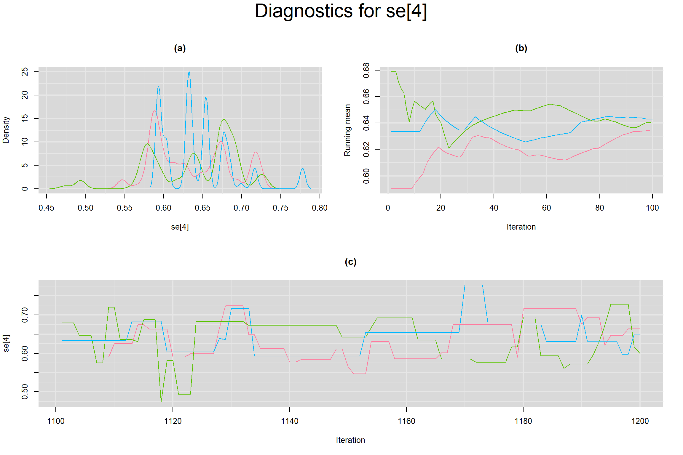
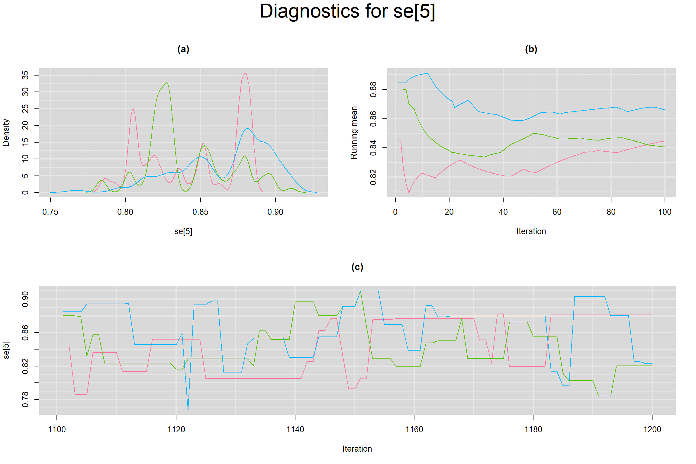
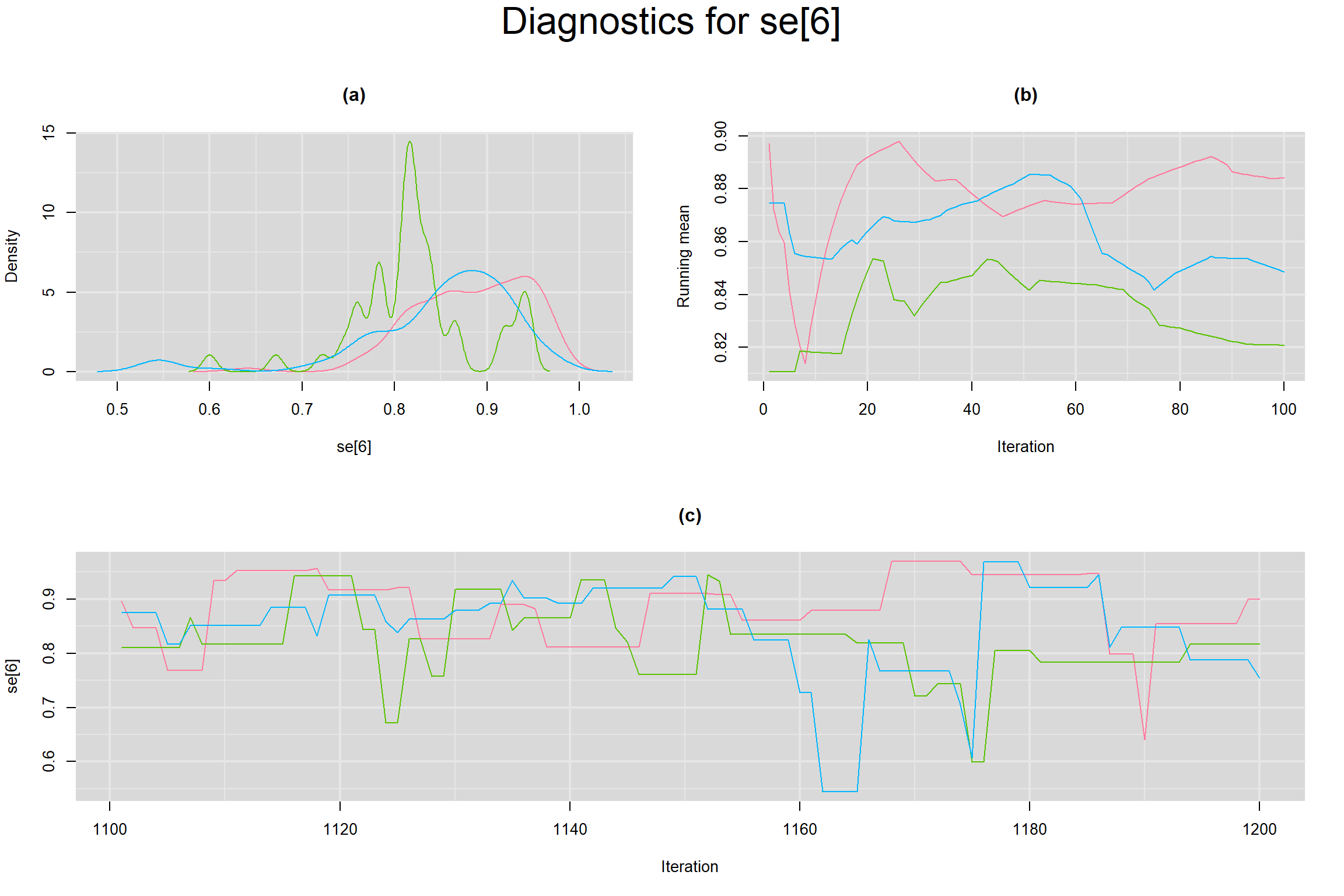
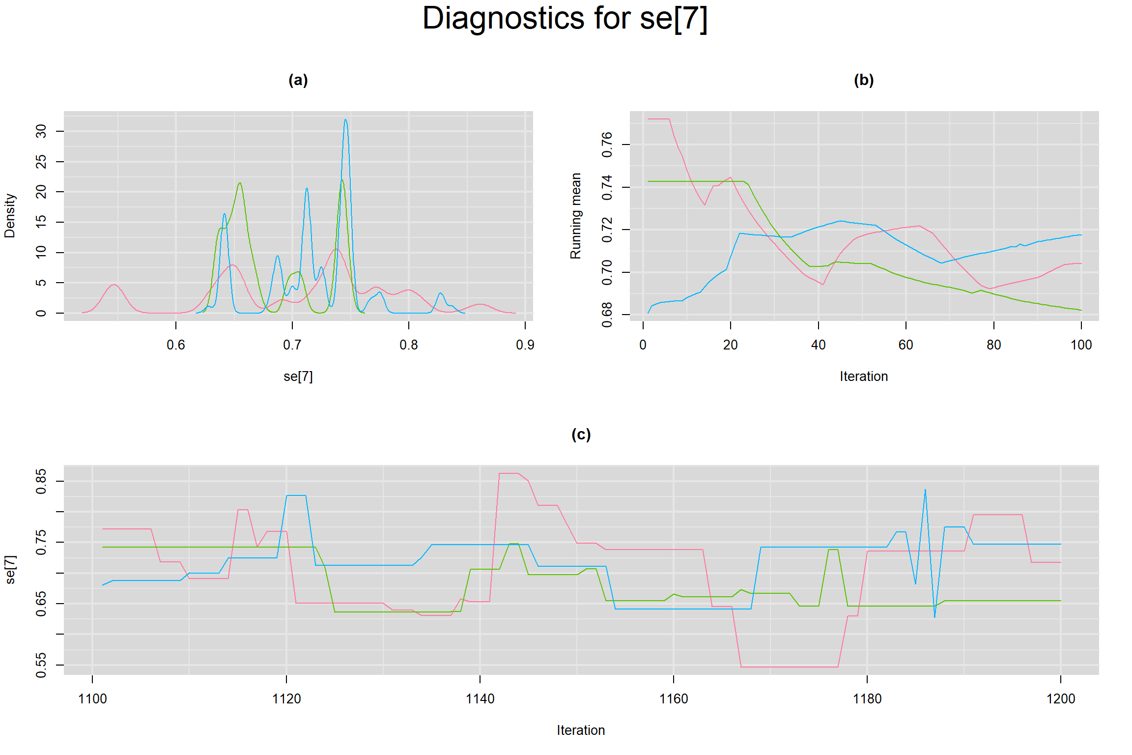
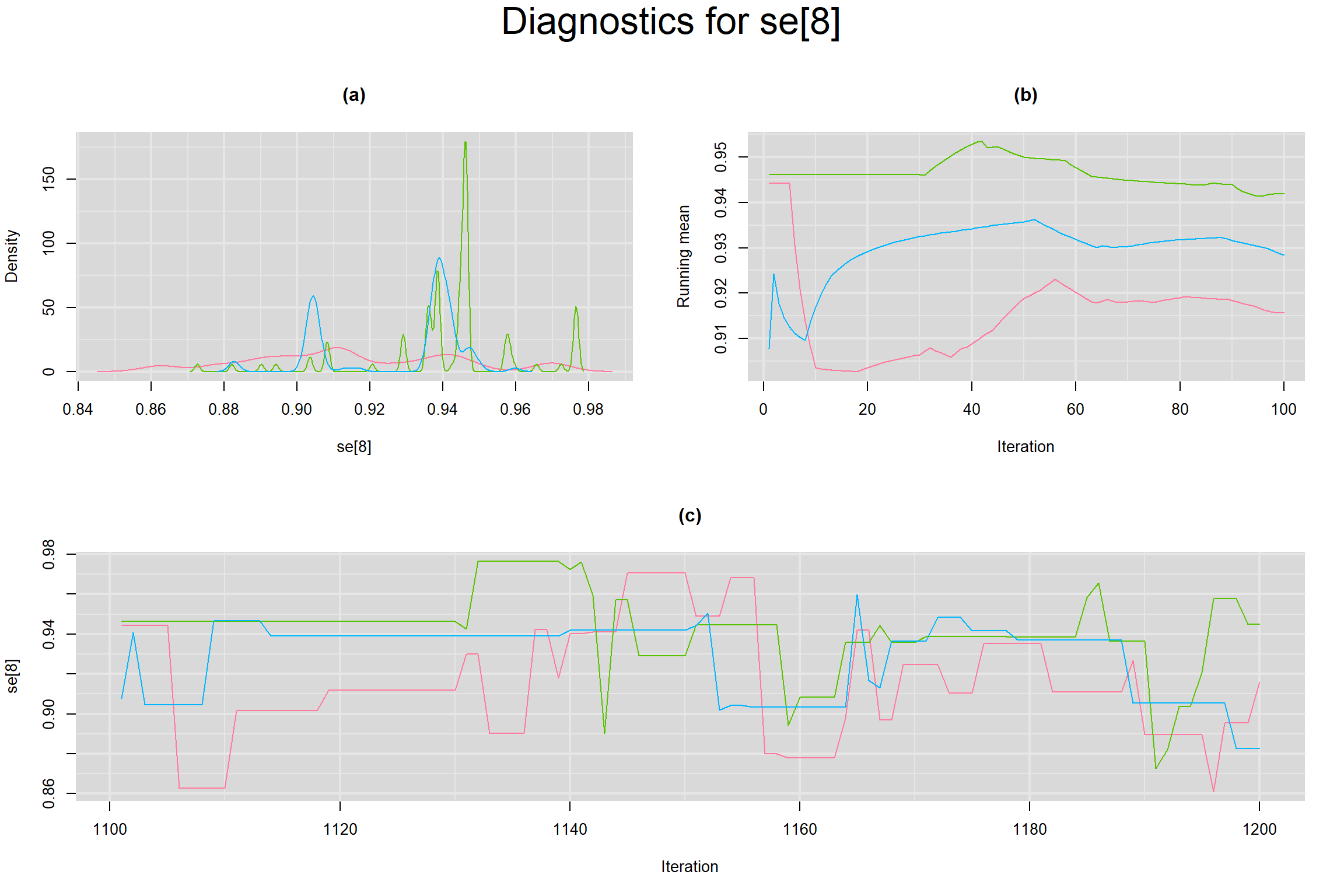
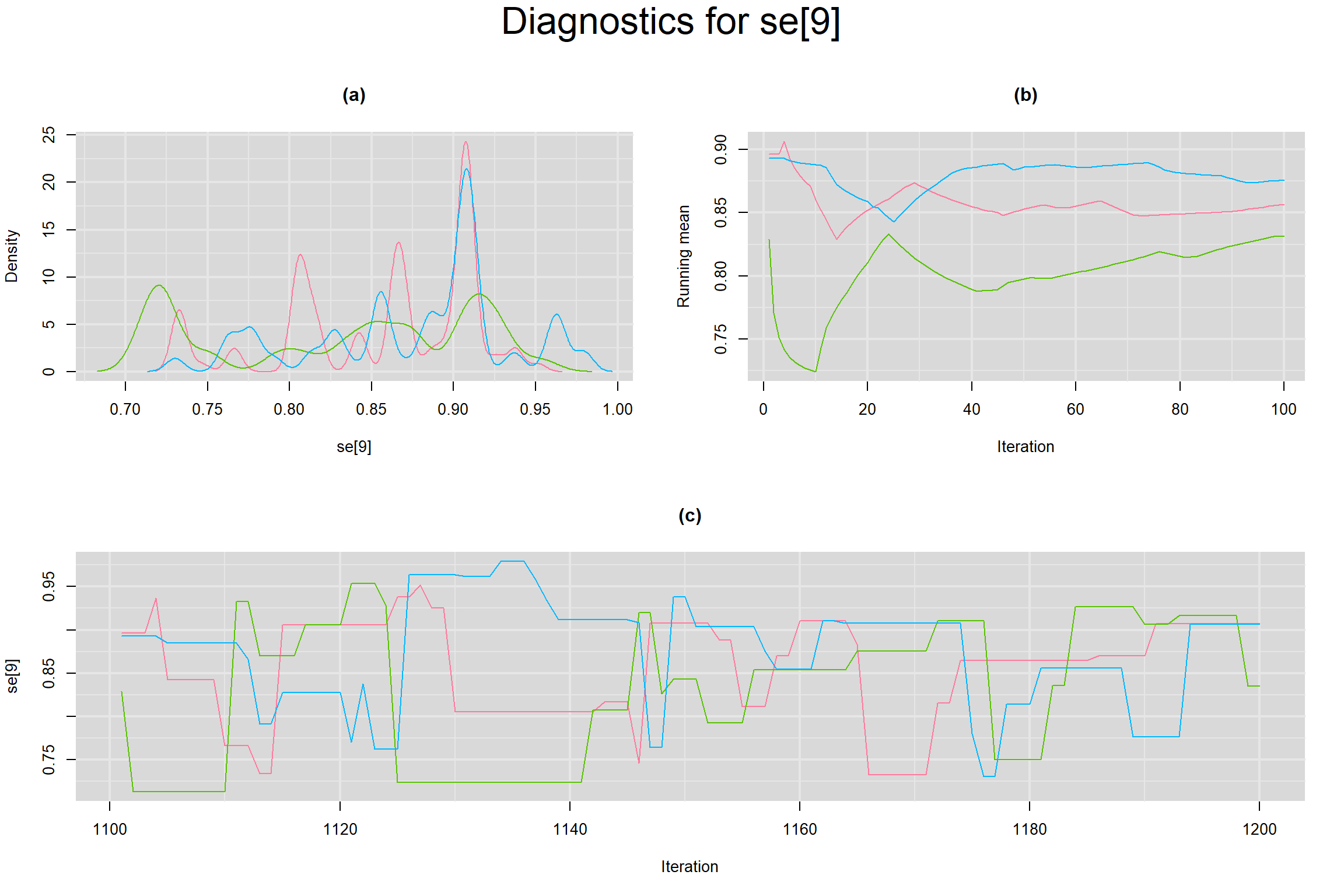
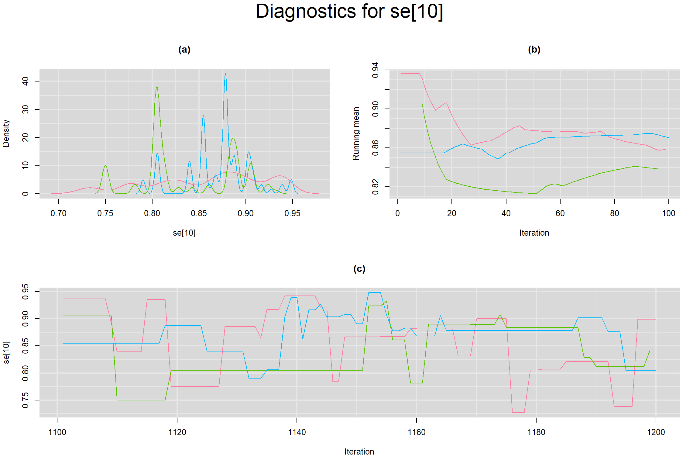
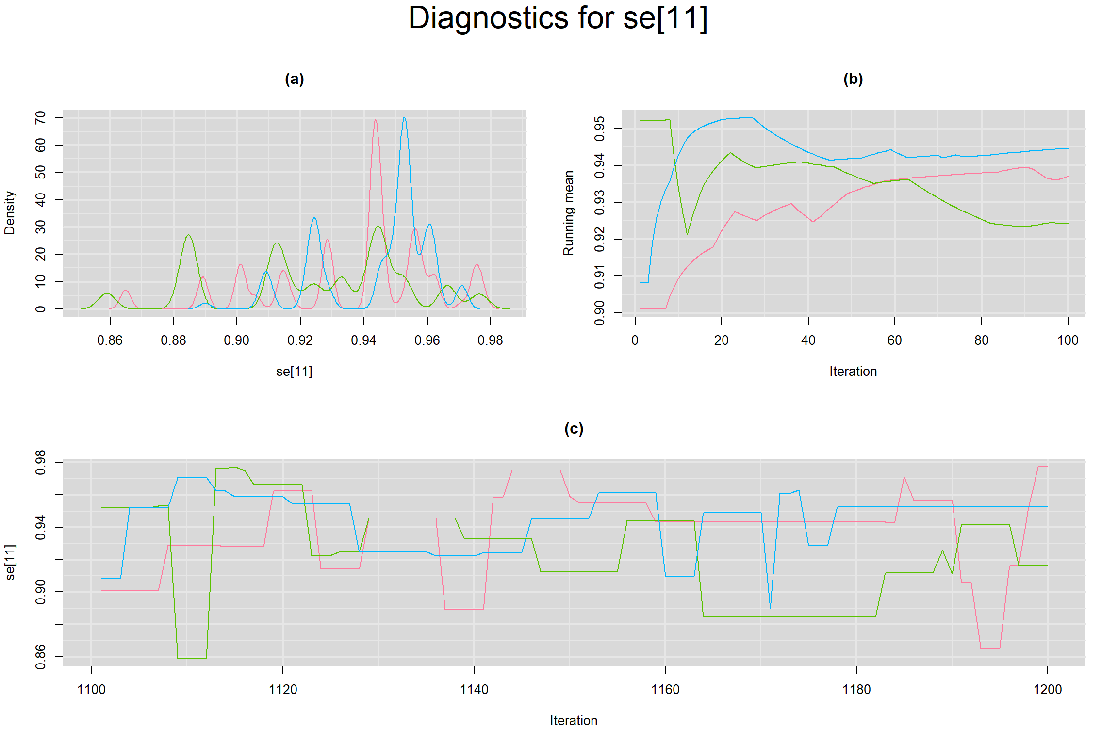
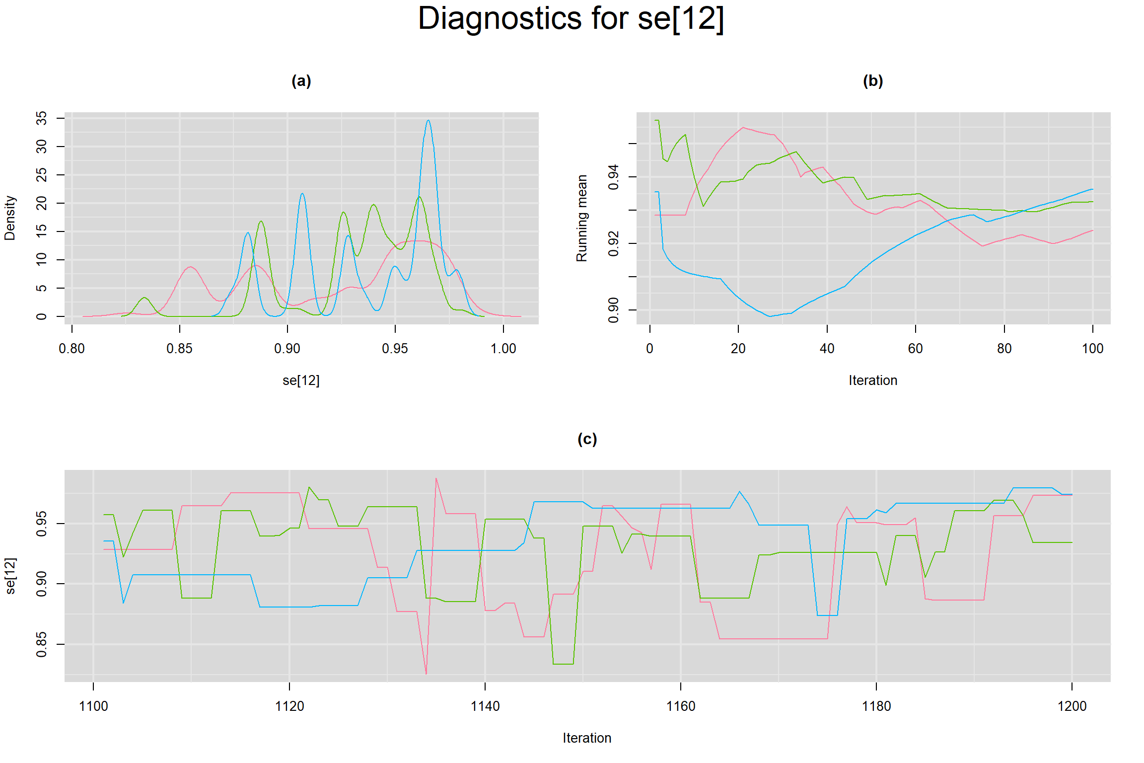
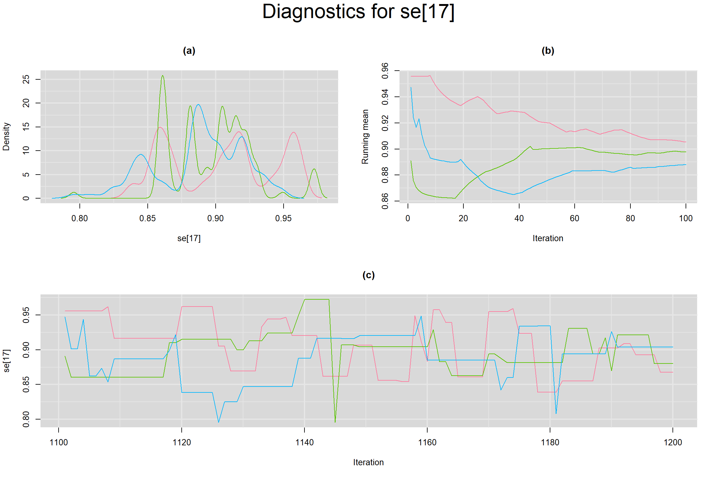
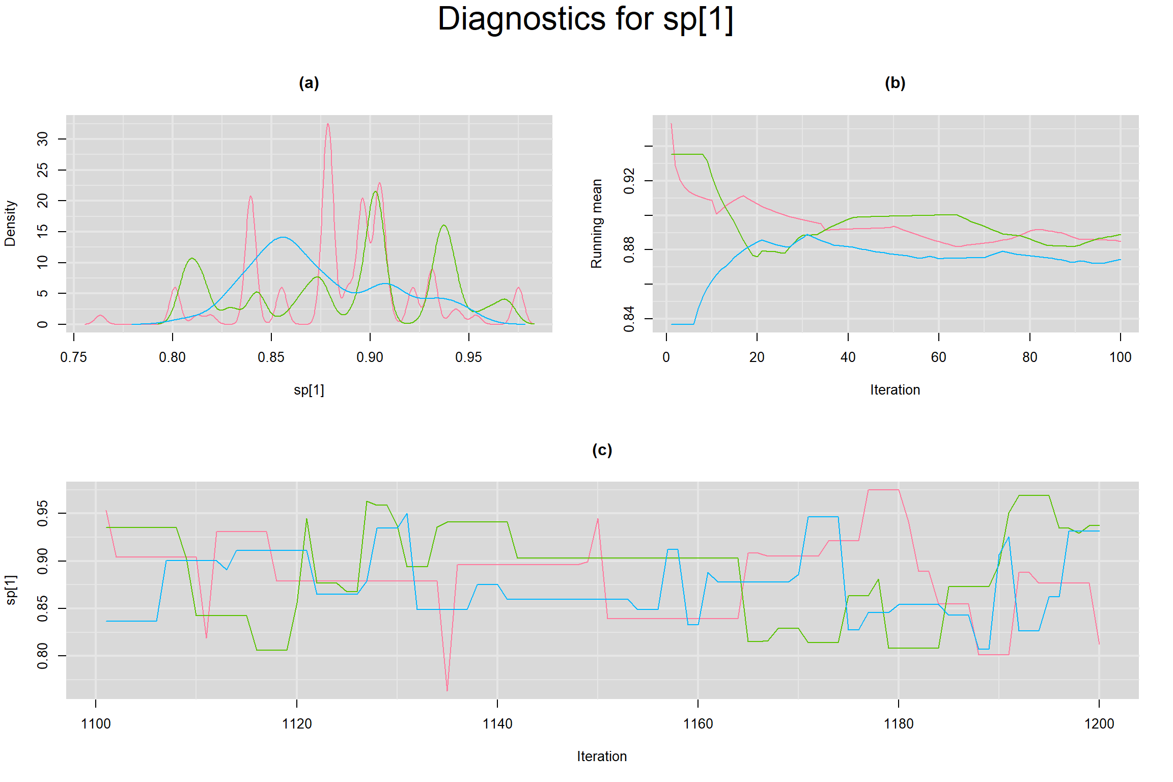
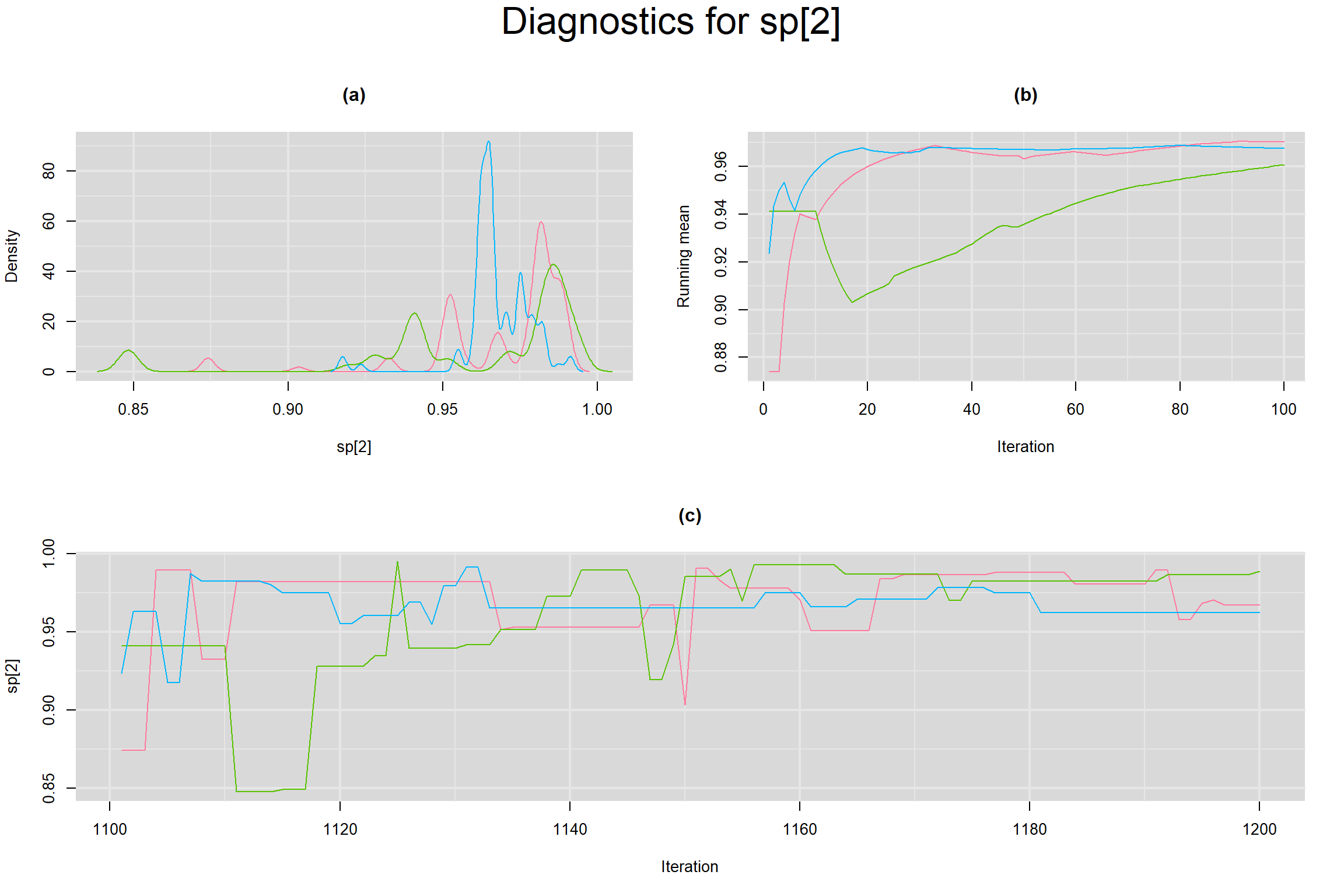
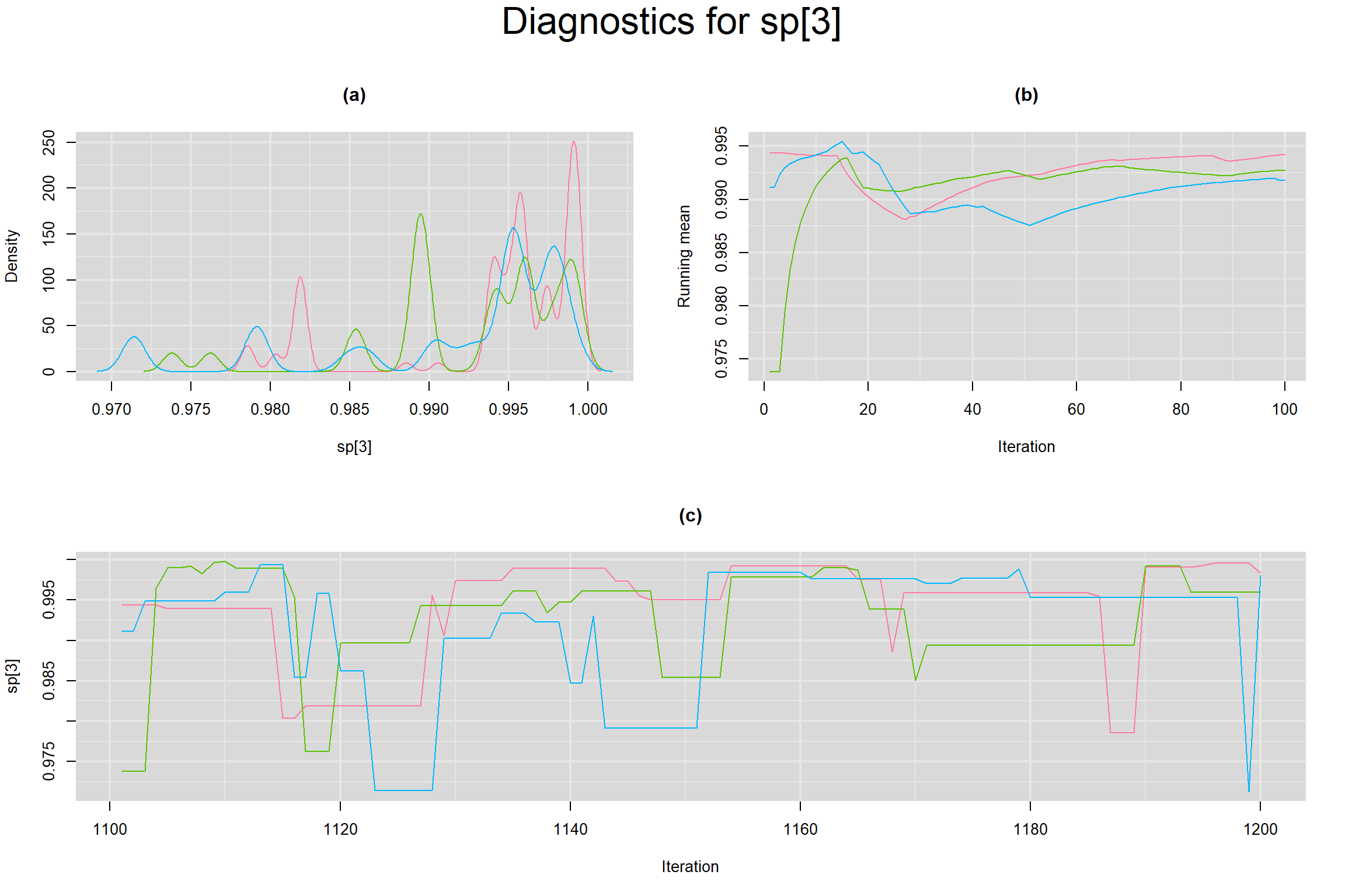
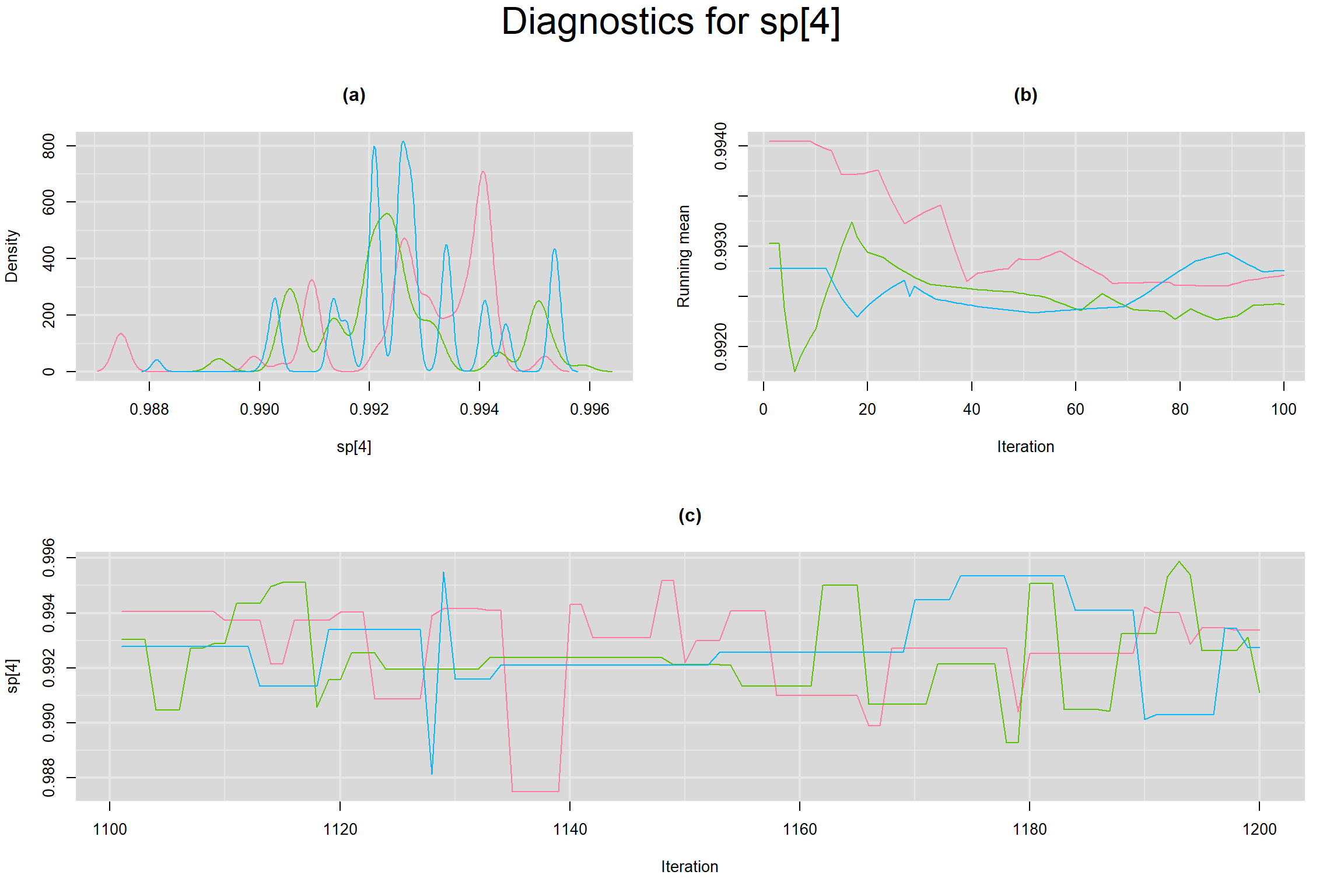
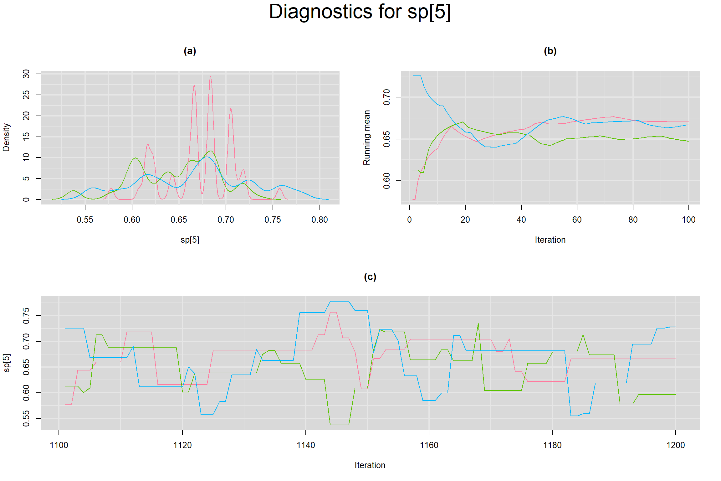
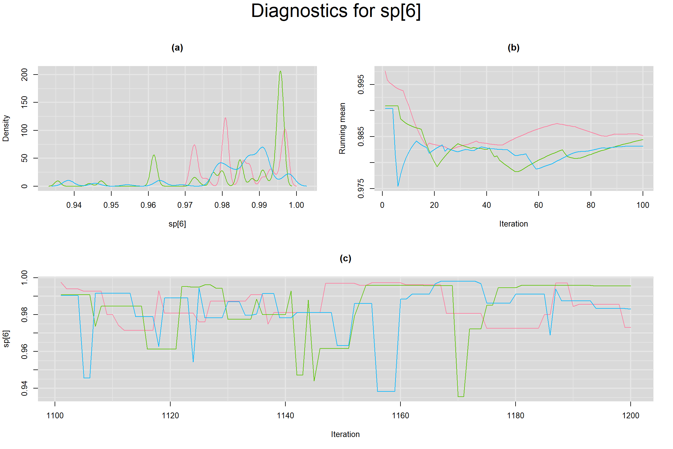
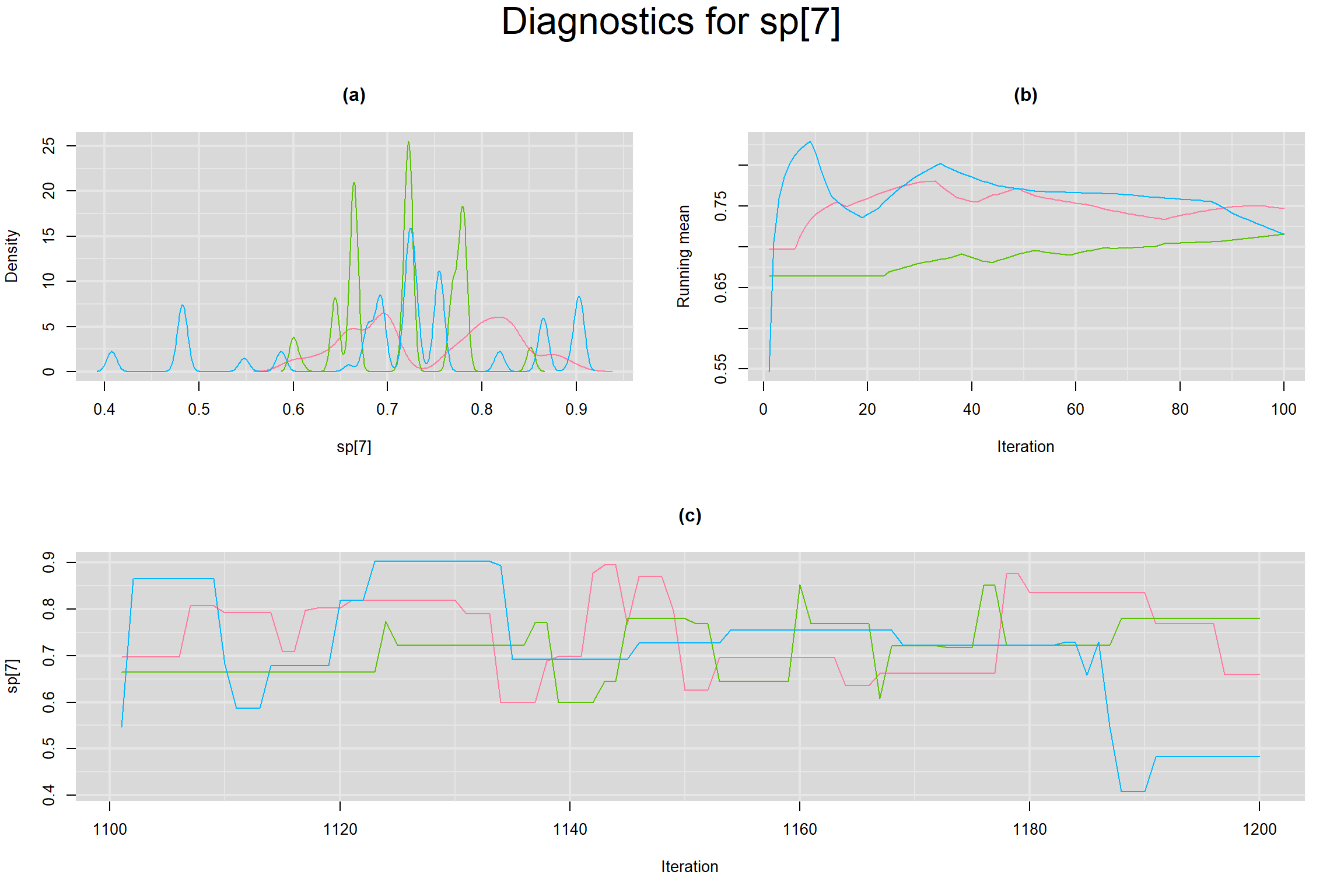
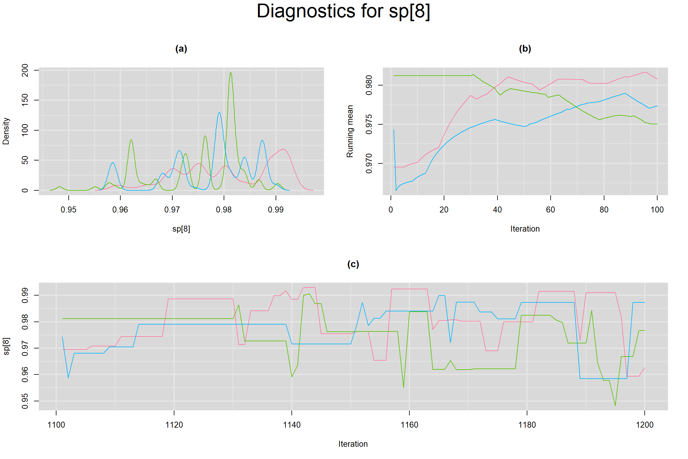
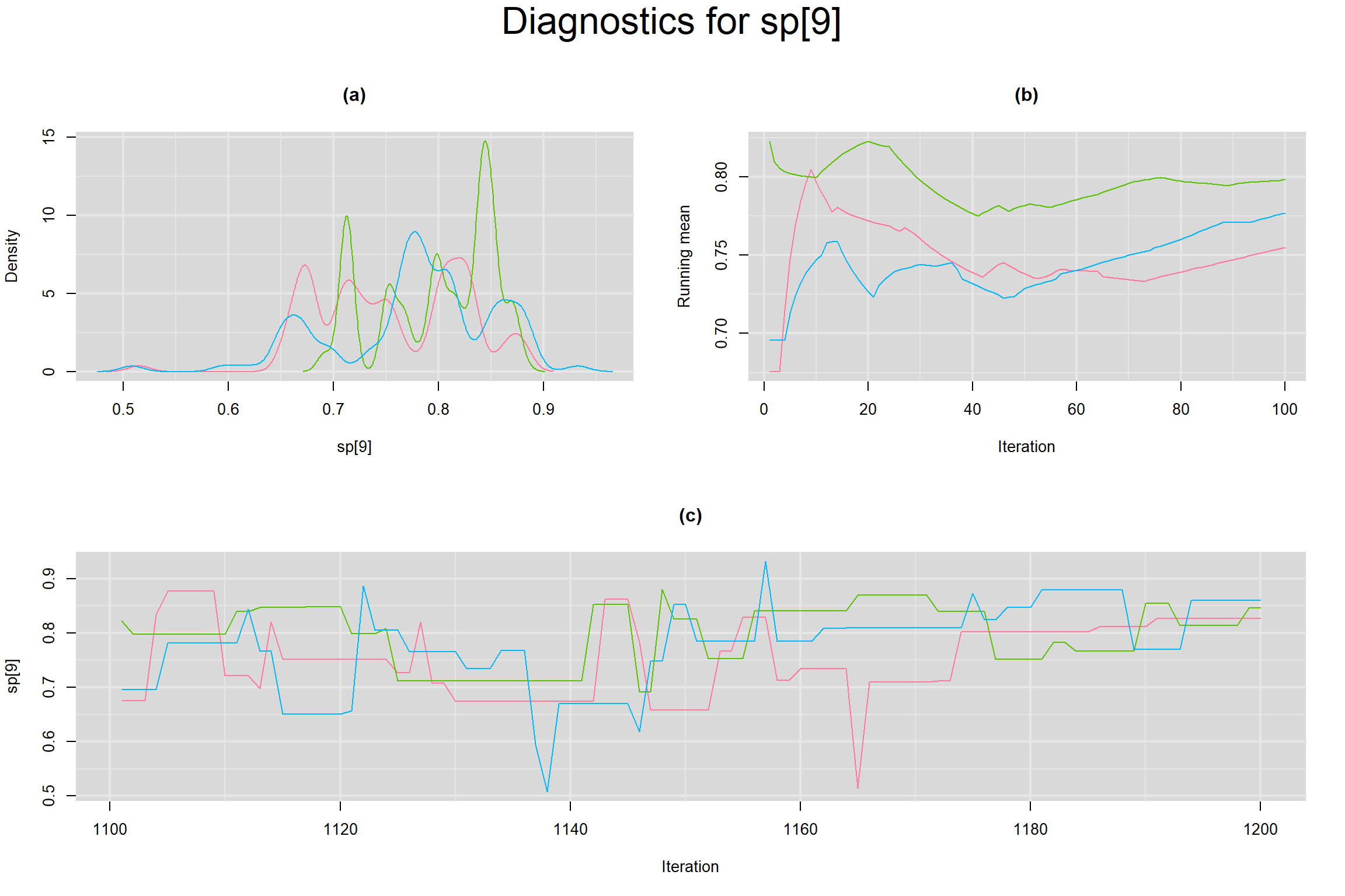
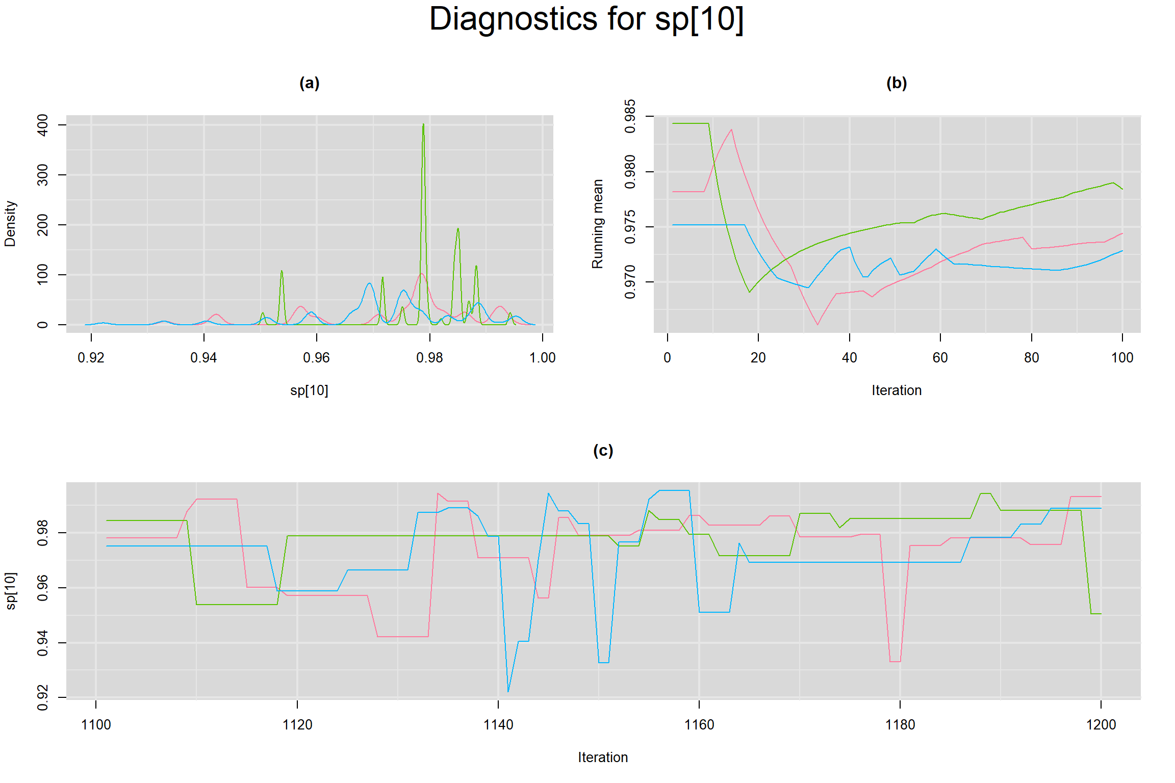
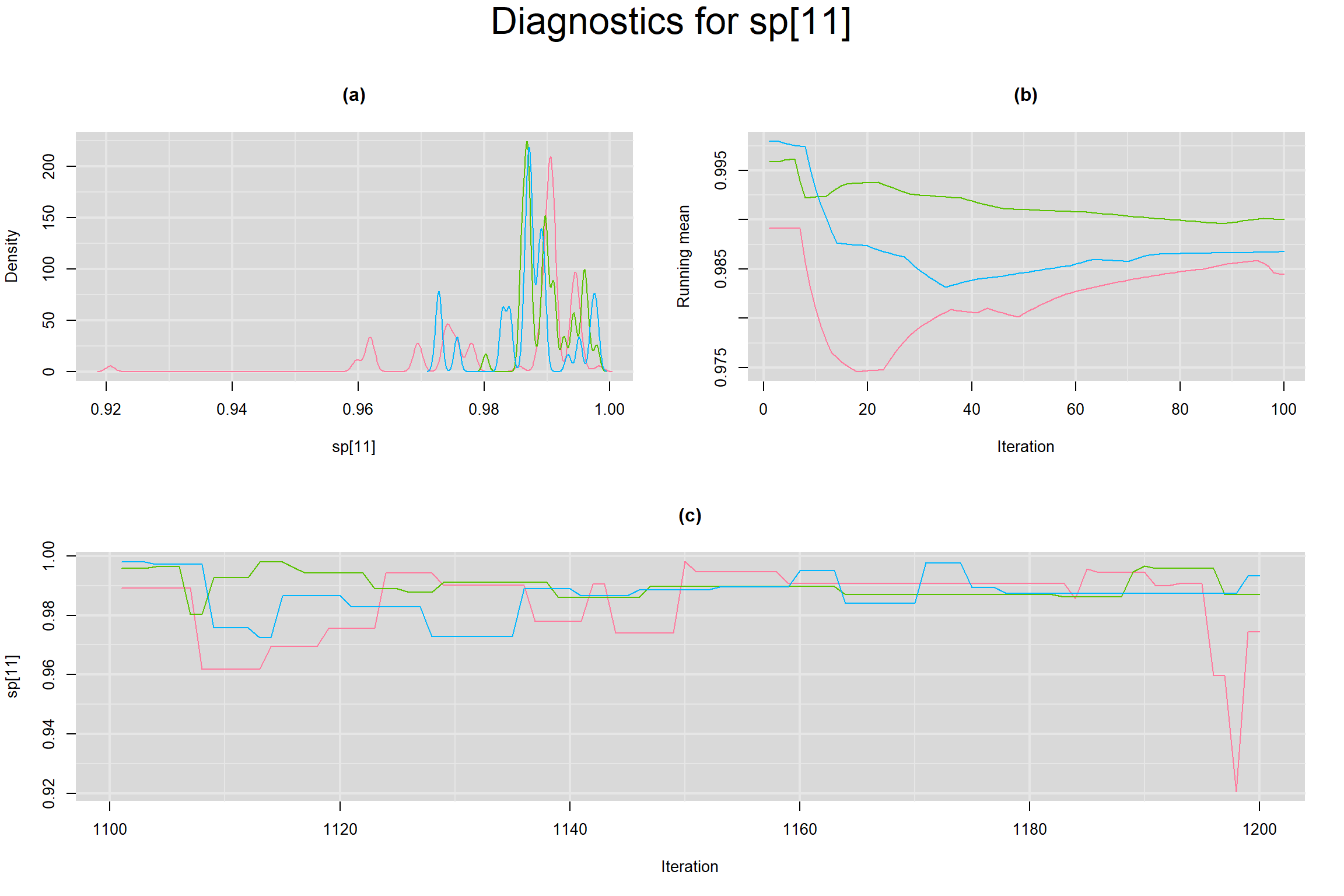
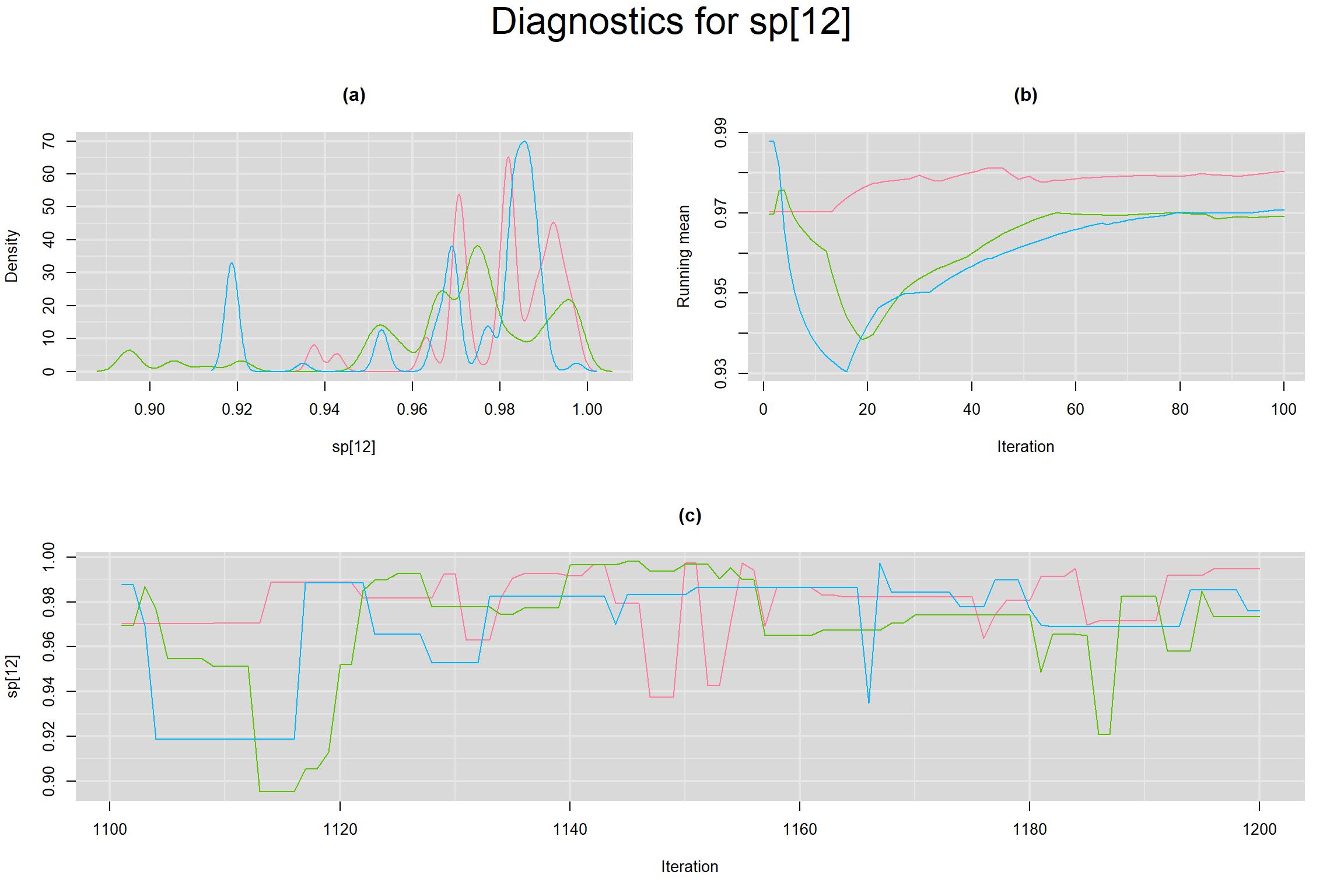
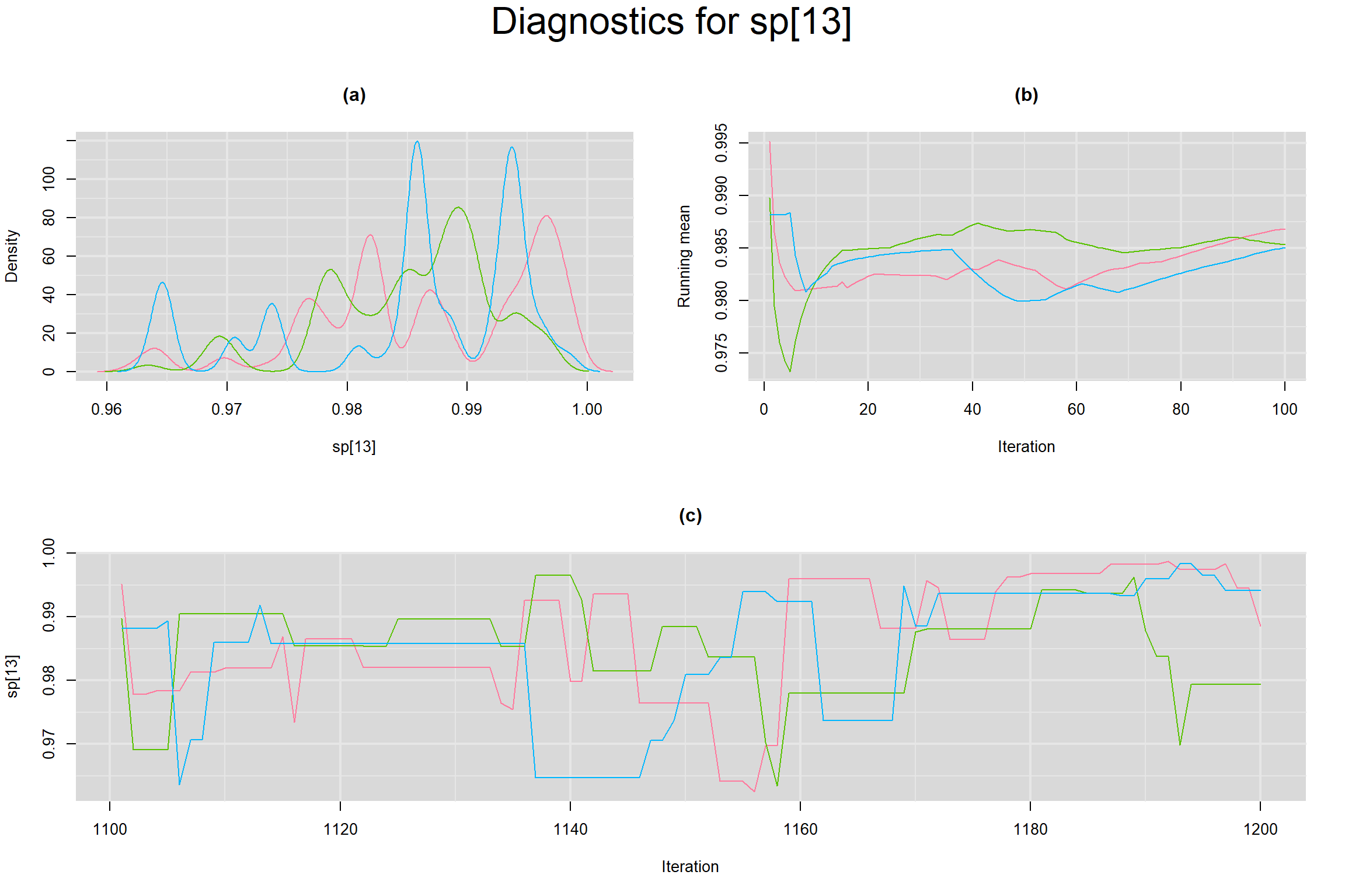
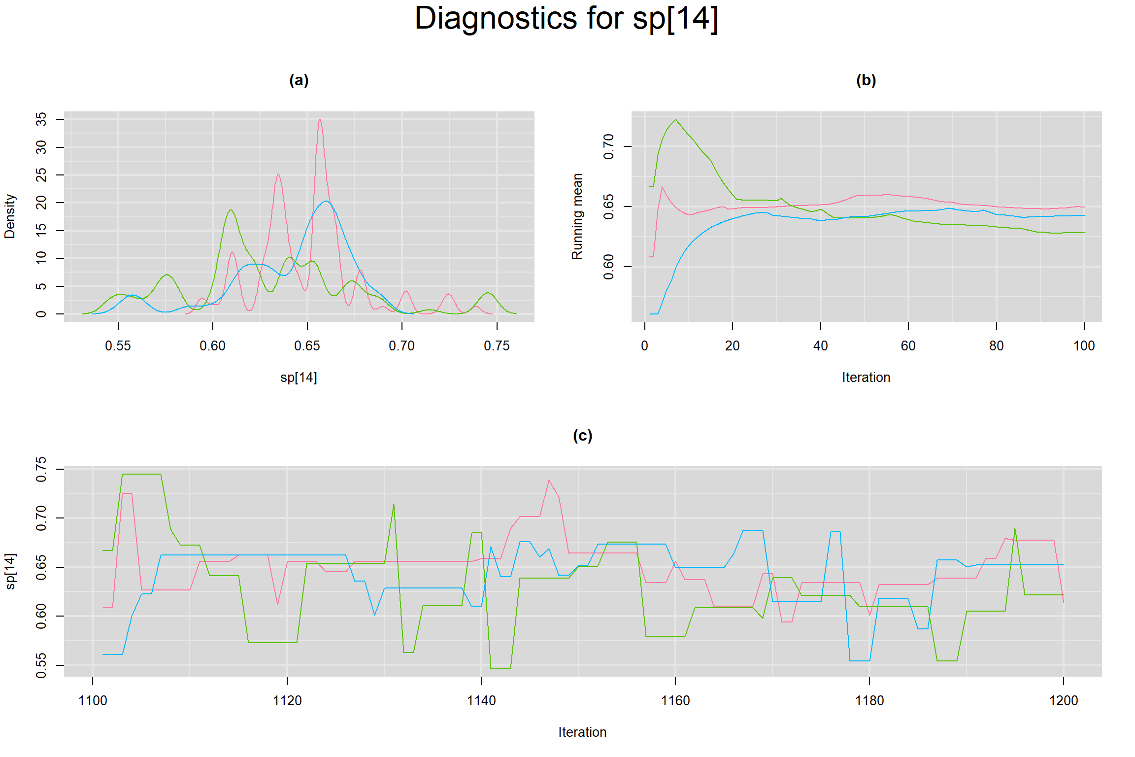
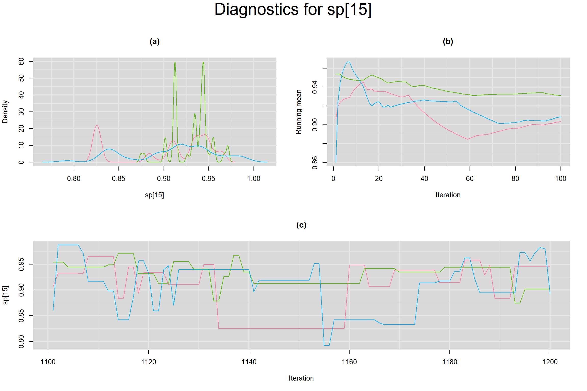
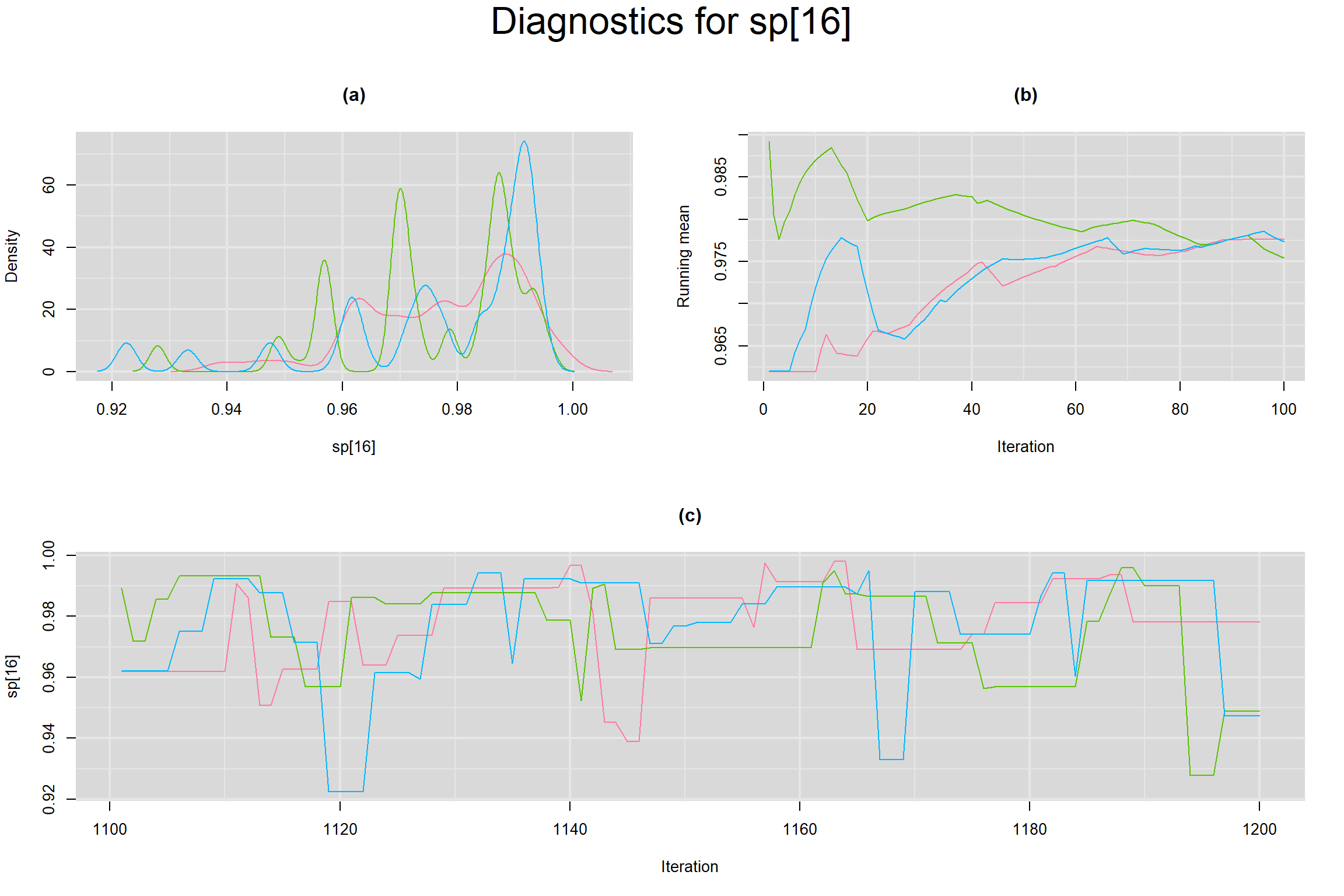
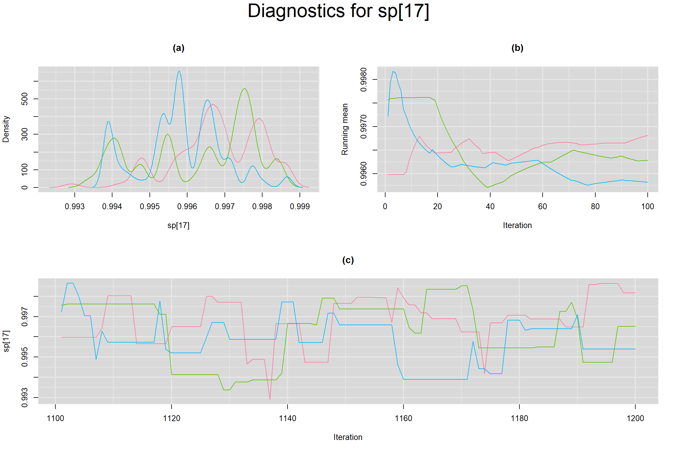
CONVERGENCE DIAGNOSTIC TOOLS
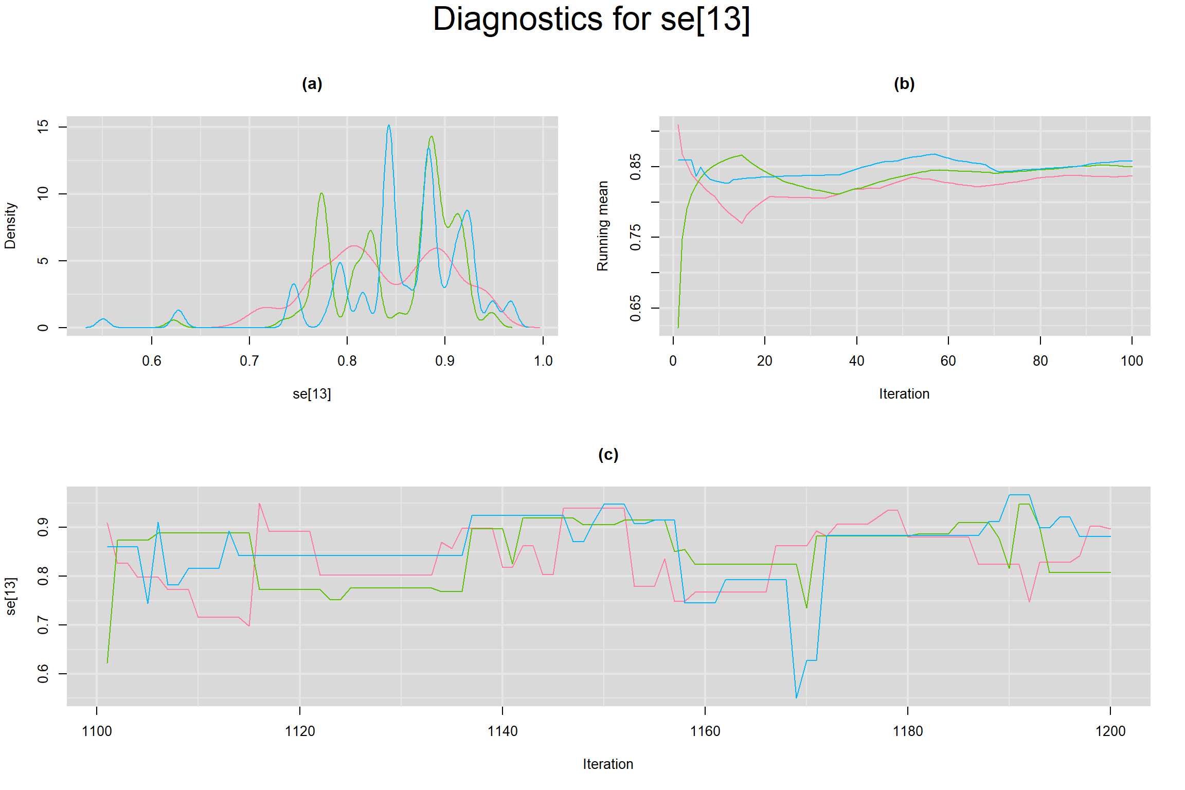
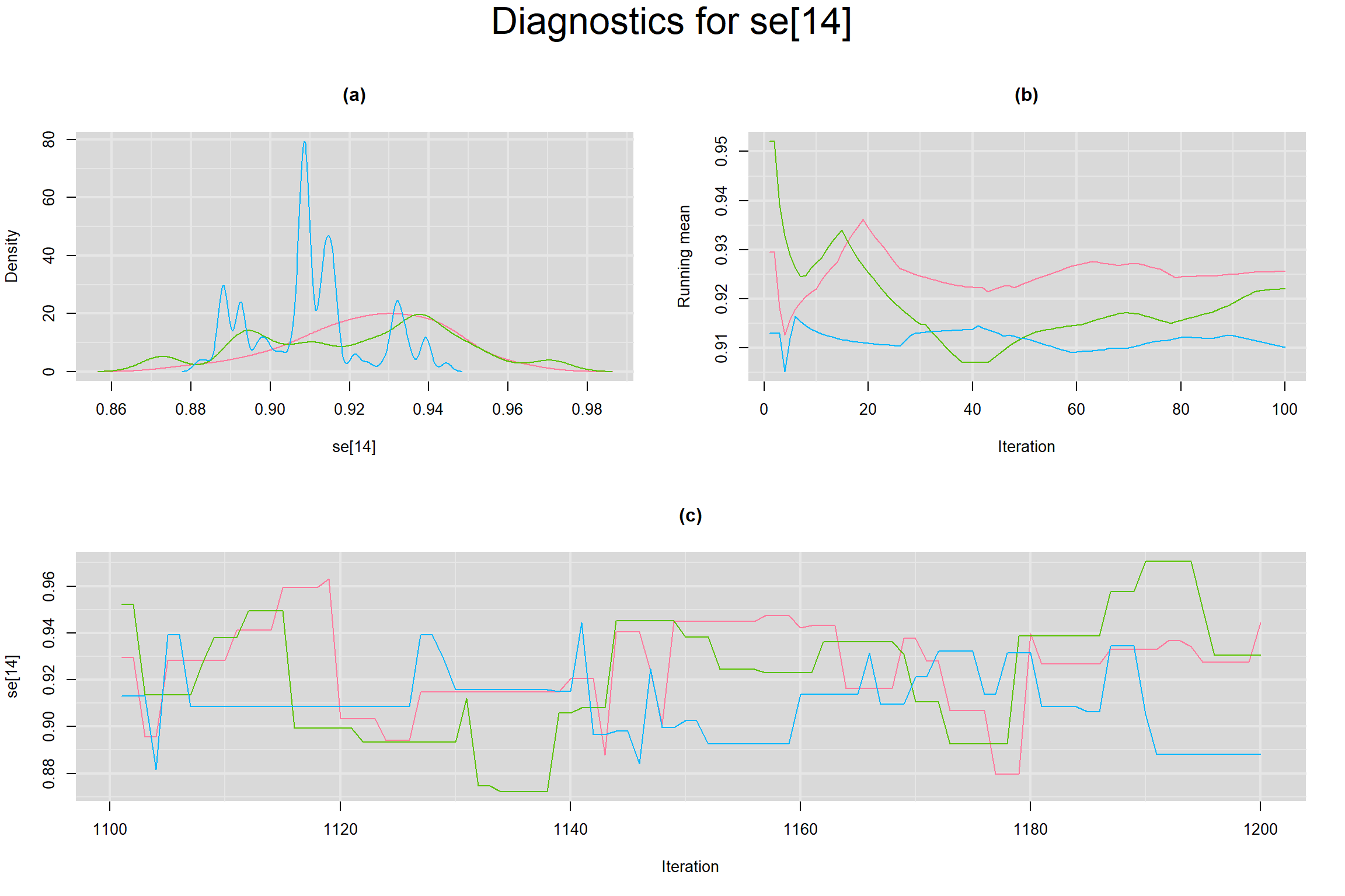
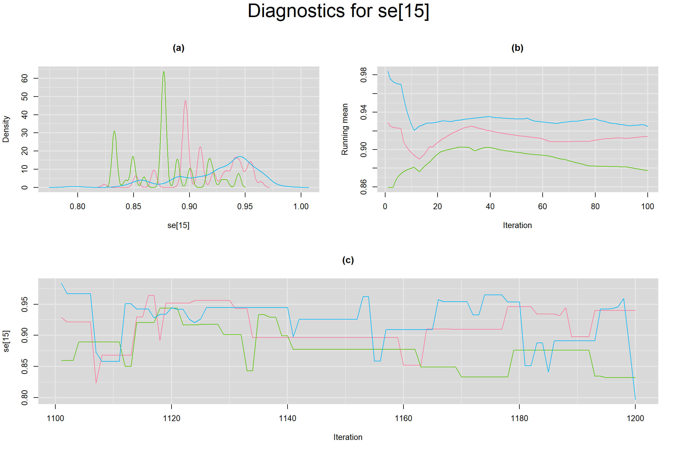
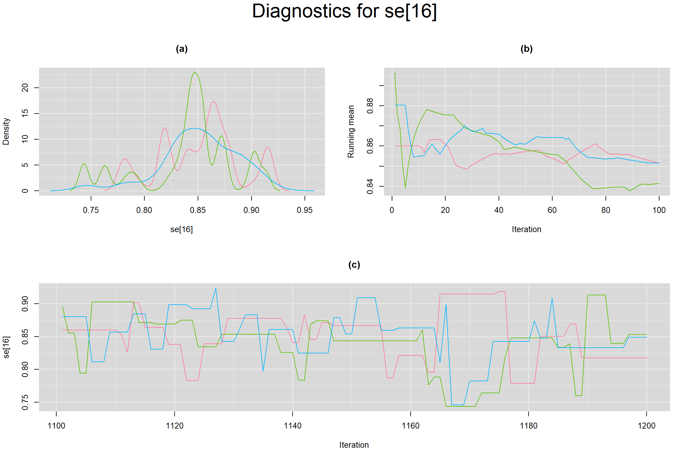
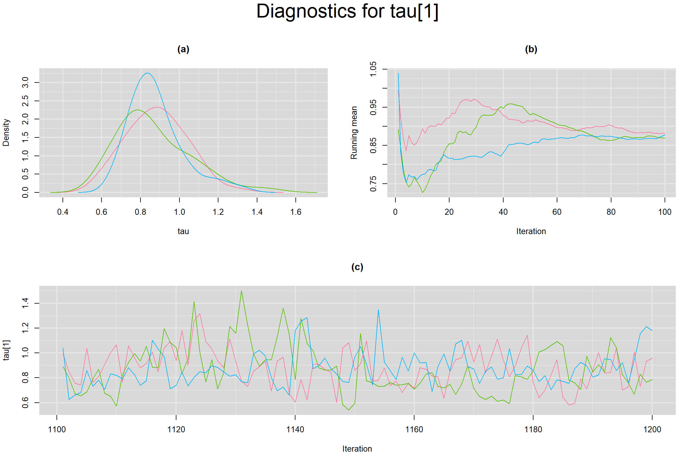
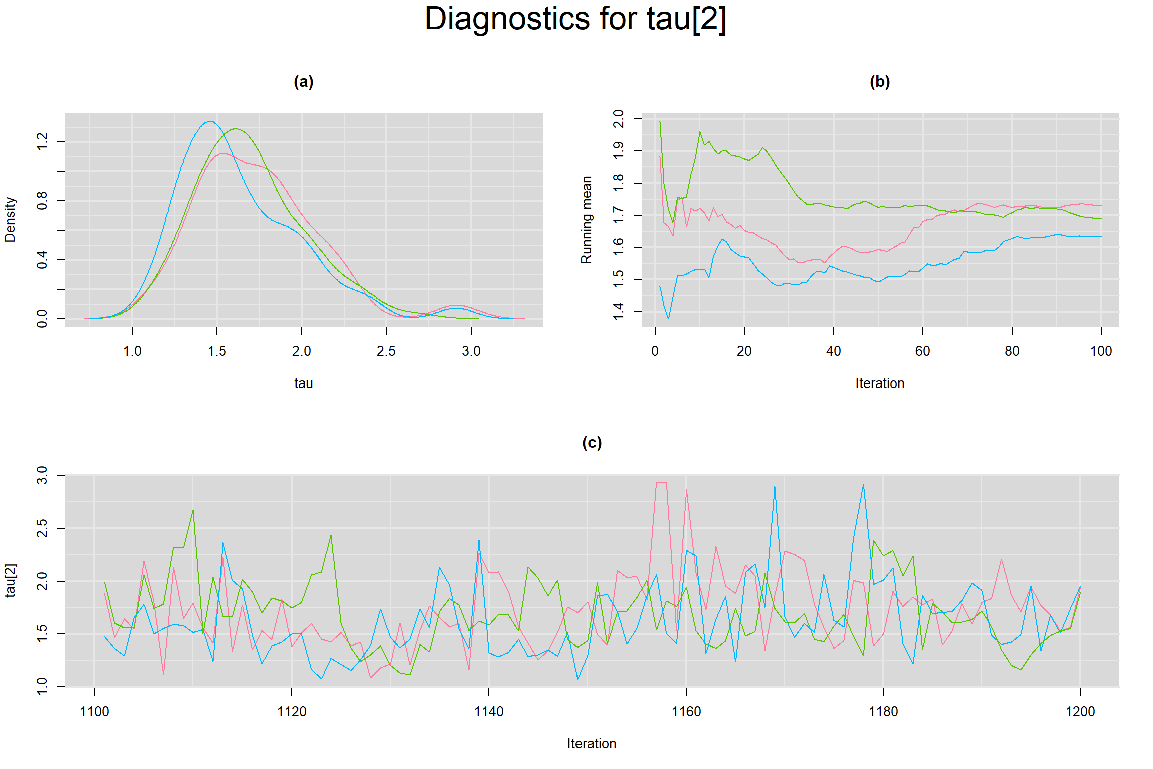
Visual inspection of convergence for key parameters can be studied below. For a given parameter, panel (a) shows posterior density plot; (b) the running posterior mean value; and (c) the history plot. Each chain is identified by a different color. Similar results from all3 chains would suggest the algorithm has converged.
PREDICTED SENSITIVITY AND SPECIFICITY IN A FUTURE STUDY
SUMMARY SENSITIVITY AND SPECIFICITY ACROSS ALL STUDIES
MEAN LOGIT-TRANSFORMED SENSITIVITY AND SPECIFICITY
CORRELATION BETWEEN MEAN LOGIT-TRANSFORMED SENSITIVITY AND MEAN LOGIT-TRANSFORMED SPECIFICITY
SENSITIVITY IN INDIVIDUAL STUDIES
SPECIFICITY IN INDIVIDUAL STUDIES
BETWEEN-STUDY VARIANCE IN THE LOGIT-TRANSFORMED SENSITIVITY AND SPECIFICITY
BETWEEN-STUDY STANDARD DEVIATION IN THE LOGIT-TRANSFORMED SENSITIVITY AND SPECIFICITY
REFERENCES
Brooks, S. P., and A Gelman. 1998. “General methods for monitoring convergence of iterative simulations.” Journal of Computational and Graphical Statistics, no. 7: 434–55.
- Butler-Laporte, G, Lawandi, A, Schiller, I, Yao, M, Dendukuri, N, McDOnald, E. G. and Lee, T. C. 2021. “Comparison of Saliva and Nasopharyngeal Swab Nucleic Acid Amplification Testing for Detection of SARS-CoV-2; A Systematic Review and Meta-analysis.” JAMA Intern Med.
Gelman, A, J. B. Carlin, H. S. Stern, D. B. Dunson, A Vehtari, and D. B. Rbin. 2013. “Bayesian Data Analysis.” Chapman & Hall/CRC Press, London, Third Edition.
Gelman, A, and D. B. Rubin. 1992. “Inference from iterative simulation using multiple sequences.” Statistical Sciences, no. 7: 457–72.
Reitsma, J. B., A. S. Glas, A. W. Rutjes, R. J. Scholten, P. M. Bossuyt, and A. H. Zwinderman. 2005. “Bivariate analysis of sensitivity and specificity produces informative summary measures in diagnostic reviews.” Journal of CLinical Epidemiology, no. 58: 892–990.