Bayesian 3-LC Random Effects Model

Authors

Ian Schiller

Nandini Dendukuri

Published

January 11, 2024

Introduction

This article is intended to give the reader basic instructions on how to run an rjags script to perform a Bayesian analysis of diagnostic test accuracy and disease prevalence in the absence of a perfect reference test in the context of a 3-latent class random effects model (Dendukuri and Wang (2009)). The script is implemented in R using the rjags package, which interfaces with the JAGS (Just Another Gibbs Sampler) software for Bayesian analysis.

The term “3-latent class” refers to the presence of three hidden or latent classes in the data by acknowledging for example that tests based on different biological mechanisms might be measuring different latent variables, which in turn are measuring the latent target condition.

Random effects are incorporated into the model to account for conditional dependence between the observed diagnostic tests.

An example dataset is provided for the user to familiarize themself with the script. It is from a study conducted to estimate the prevalence of Chlamydia trachomatis infection among a group of women (Black and Martin (2002)).

Download `rjags` Script

The full script, can be downloaded here.

Script Instructions

Suggested `R Package`

Below is a list of packages we recommend installing. Aside from rjags, which is mandatory, the other packages are optional when performing LC analysis. We do recommend them as they are used in the script. Be aware that some functionalities of the script may not work if you do not install every packages listed below.

require(rjags)     # PACKAGE TO RUN THE jags MODEL. MANDATORY
require(MCMCvis)   # THIS PACKAGE CONTAINS THE MCMCsummary FUNCTION USED IN THIS SCRIPT
require(mcmcplots) # USED FOR THE CREATION OF THE CONVERGENCE PLOTS
require(DT)        # THIS LIBRARY ALLOWS A NICE DATA DISPLAY WITH THE SEARCH BAR OPTION.
require(dplyr)     # TO SETUP THE DATASET IN A SUITABLE FORMAT FOR rjags ANALYSIS 
require(rBeta2009) # TO GENERATE INITAL VALUES FOR LATENT CLASS PROBABILITIES
require(truncnorm) # TO GENERATE INITIAL VALUES FOR SPECIFICITY OF CUTLURE TEST BASED ON PRIOR

C.trachomatis Dataset

The C.trachomatis dataset is taken from a study conducted to estimate the prevalence of Chlamydia trachomatis infection among a group of women). It includes 3551 participants with results on 3 diagnostic tests as follow

Ligase chain reaction (LCR)
Polymerase chain reaction (PCR)
DNA probe test (DNAP)
Culture test

Positive tests are represented by the value 1, while negative tests are noted 0. Each row of the data represents one of the 16 possible cross-classification result of the 4 tests. The last column is the observed frequencies of the 16 cross-classification results.

We recommend to save the C.trachomatis dataset in a .txt extension file as C.trachomatis.txt in the same folder as the script. The data can be uploaded with the read.table function.

DATA <- read.table("C_trachomatis.txt", header=TRUE)
datatable(DATA, extensions = 'AutoFill')#, options = list(autoFill = TRUE))

This data formatting is however not compatible with the model we will write below, as we need to express the data on an individual level (one row corresponding to one patient) and store it in a list we call dataList. The data that will be included in dataList are the sample size, noted N, the number of latent class L and the actual joint test results of each individual subject, noted y.

# Joint test results for each patient (each row represents a different patient and each column represents a test result)
y <- DATA %>%  
  slice(rep(seq_len(n()), Obs_Freq)) %>% 
  select(-Obs_Freq)
# Total number of patients
N = dim(y)[1]
dataList <- list(y=y, N=N, L=3)

As seen below, the data y contains as many rows as there are subjects and all 4 columns represent the subejct’s test results.

datatable(y, extensions = 'AutoFill')#, options = list(autoFill = TRUE))

Bayesian Latent Class Random Effects Model

The LCR and PCR tests are nucleic-acid amplification tests (NAATs) which are designed to measure the presence of C. trachomatis DNA, which means those tests cannot distinguish between viable and nonviable bacteria. The culture test is designed to measure viable C. trachomatis bacteria. The DNAP test is also designed to measure C. trachomatis DNA, but unlike the NAATs test, it is less likely to detect nonviable bacteria. Therefore Dendukuri and Wang (2009) hypothesized that LCR and PCR tests would measure the DNA latent variable which is a proxy for the true disease status, while DNAP and culture tests would measure viable C. trachomatis latent variable (further referred to as the disease latent variable). The diagram below is a visual representation of a multiple latent variable for the Chlamydia trachomatis tests, where the rectangles represent the observed variables and the ovals represent the latent variables.

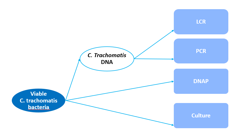
The 2 latent variables C. trachomatis DNA (l1) and viable C. trachomatis bacteria (D) allows for 4 possible latent classes:

Latent class 1 (LC1): l1 positive and D positive
Latent class 2 (LC2): l1 positive and D negative
Latent class 3 (LC3): l1 negative and D negative
Latent class 4 (LC4): l1 negative and D positive

It was hypothesized that LC4 is not possible, i.e. there cannot be viable C. trachomatis bacteria without the presence of C. trachomatis DNA. This class was therefore excluded and the model was reduced to a 3-latent class model.

Implementing the Bayesian 3-latent class random effects model in rjags involves specifying the priors and likelihood. Markov Chain Monte Carlo (MCMC) methods, such as Gibbs sampling, are then employed to estimate the posterior distribution of the model parameters.

The rjags model is saved on the current directory (where your script and data should already be saved ideally) as model.txt. Below is the model following the JAGS syntax.

modelString =  
  "model {

for (i in 1:N) {

  #============
  # LIKELIHOOD 
  #============
  
    for (j in 1:4) {
      y[i, j] ~ dbin(p[LC[i],i, j], 1)
    }
    
    LC[i] ~ dcat(pLC[1:L])
    r[i] ~ dnorm(0,1)
    
    #===========================================================================
    # Conditional probability of a positive observation for a given latent class
    #===========================================================================
    # LATENT CLASS L1 : viable C. trachomatis bacteria positive (D+) and true DNA status positive (l1+)
    p[1, i, 1] <- phi(a[1, 1] + b.RE[1] * r[i])
    p[1, i, 2] <- phi(a[1, 2] + b.RE[2] * r[i])
    p[1, i, 3] <- phi(a[1, 3])
    p[1, i, 4] <- phi(a[1, 4])
    
    # LATENT CLASS L2 : viable C. trachomatis bacteria negative (D-) and true DNA status positive (l1+)
    p[2, i, 1] <- phi(a[2, 1])
    p[2, i, 2] <- phi(a[2, 2])
    p[2, i, 3] <- phi(a[2, 3])
    p[2, i, 4] <- phi(a[2, 4])  
    
    # LATENT CLASS L3 : viable C. trachomatis bacteria negative (D-) and true DNA status negative (l1-)
    p[3, i, 1] <- phi(a[3, 1])
    p[3, i, 2] <- phi(a[3, 2])
    p[3, i, 3] <- phi(a[3, 3])
    p[3, i, 4] <- phi(a[3, 4])
    
    # LATENT CLASS 4 : viable C. trachomatis bacteria positive (D+) and true DNA status negative (l1-)
    # This latent class is assumed to be not possible
}

#==================================================
# Prior distributions
#==================================================

a[1,1] ~ dnorm(0,1)
a[1,2] ~ dnorm(0,1)
a[1,3] ~ dnorm(0,1)
a[1,4] ~ dnorm(0,1)

a[2,1]  <- a[1,1]
a[2,2]  <- a[1,2]
a[2,3]  ~ dnorm(0,1)
a[2,4]  ~ dnorm(0,1)T(-5, -2.05)

a[3,1]  ~ dnorm(0,1) 
a[3,2]  ~ dnorm(0,1)
a[3,3]  <- a[2,3]
a[3,4]  <- a[2,4]
    
b.RE[1] ~ dnorm(0,1)I(0,)
b.RE[2] <- b.RE[1]

pLC[1:L] ~ ddirch(prior[1:L])
for (i in 1:L) {
  prior[i]<-1
}

#=========================================================
# Other parameters of interest 
#=========================================================

# SENSITIVITY/SPECIFICITY WITH RESPECT TO viable C. trachomatis bacteria
se_D[1] <- phi(a[1, 1]/sqrt(1 + b.RE[1] * b.RE[1]))
se_D[2] <- phi(a[1, 2]/sqrt(1 + b.RE[2] * b.RE[2]))
se_D[3] <- phi(a[1, 3])
se_D[4] <- phi(a[1, 4])

sp_D[1] <- ( phi(-a[2, 1])*pLC[2] + phi(-a[3, 1])*pLC[3] )/(pLC[2]+pLC[3])
sp_D[2] <- ( phi(-a[2, 2])*pLC[2] + phi(-a[3, 2])*pLC[3] )/(pLC[2]+pLC[3])
sp_D[3] <- ( phi(-a[2, 3])*pLC[2] + phi(-a[3, 3])*pLC[3] )/(pLC[2]+pLC[3])
sp_D[4] <- ( phi(-a[2, 4])*pLC[2] + phi(-a[3, 4])*pLC[3] )/(pLC[2]+pLC[3])


# SENSITIVITY/SPECIFICITY WITH RESPECT TO true DNA status
se_l1[1] <- ( phi(a[1, 1]/sqrt(1 + b.RE[1] * b.RE[1]))*pLC[1] + phi(a[2, 1]/sqrt(1 + b.RE[1] * b.RE[1]))*pLC[2] )/(pLC[1]+pLC[2])
se_l1[2] <- ( phi(a[1, 2]/sqrt(1 + b.RE[2] * b.RE[2]))*pLC[1] + phi(a[2, 2]/sqrt(1 + b.RE[2] * b.RE[2]))*pLC[2] )/(pLC[1]+pLC[2])
se_l1[3] <- ( phi(a[1, 3])*pLC[1] + phi(a[2, 3])*pLC[2] )/(pLC[1]+pLC[2])
se_l1[4] <- ( phi(a[1, 4])*pLC[1] + phi(a[2, 4])*pLC[2] )/(pLC[1]+pLC[2])

sp_l1[1] <- phi(-a[3, 1])
sp_l1[2] <- phi(-a[3, 2])
sp_l1[3] <- phi(-a[3, 3])
sp_l1[4] <- phi(-a[3, 4])

# PREVALENCE OF viable C. trachomatis bacteria
prev <- pLC[1]

# PREVALENCE OF true DNA status
prev_DNA <- pLC[1]+pLC[2]

}"

writeLines(modelString,con="model.txt")

Prior Distributions

The prior distributions used in the script are inspired from those provided in Dendukuri and Wang (2009).

A Dirichelt(1,1,1) prior distribution was used for the 3 latent class prevalence parameters which is equivalent to a vague prior.

In a random effects model, prior distributions need to be placed on the parameters of the random effects. In the *C. Trachomatis* example, it was done by specifying \(N(0,1)\) vague priors for the a parameters and a truncated normal \(N(0,1)I(0,1)\) vague priors for the b parameters.

Further constrains were placed on the a parameters to reflect the 3-latent class structure and the fact that not all tests were designed to measure the same latent variable.

An informative prior distribution was used to reflect that the specificity of culture test is believed to lie somewhere between 98% and 100%. This was done by truncating the \(N(0,1)\) prior distribution of the a parameter associated to the specificity of culture test.

Initial Values

Initial values are needed as the starting point for estimating and updating parameters of the model in rjags. We strongly encourage the user to provide their own method of generating initial values rather than counting on rjags to generate them. Initial values can be provided in different ways in rjags. We propose one method below based on the creation of a home made function to randomly generate initial values based on the prior distributions. For more options on how to provide initial values, please see A guide on how to provide initial values in rjags

# Initial values
GenInits  = function(){  
  a11 <- rnorm(1,0,1)
  a12 <- rnorm(1,0,1)
  a13 <- rnorm(1,0,1)
  a14 <- rnorm(1,0,1)
  a21 <- a11
  a22 <- a12
  a23 <- rnorm(1,0,1)
  a24 <- rtruncnorm(1,-5,-2.05,0,1)
  a31 <- rnorm(1,0,1)
  a32 <- rnorm(1,0,1)
  a33 <- a23
  a34 <- a24
  b1 <- abs(rnorm(1,0,1))
  b2 <- b1
  pLC <- rdirichlet(1,c(1,2,3))
  
  b.RE <- c(b1, b2)
  a <- matrix(c(a11, a12, a13, a14,
                a21, a22, a23, a24,
                a31, a32, a33, a34), byrow=TRUE, ncol=4)
  pLC <- as.vector(pLC)
  
  
  list(
    a = a,
    pLC = pLC,
    b.RE = b.RE,
    .RNG.name="base::Wichmann-Hill",
    .RNG.seed=321
  )  
}

Below we use our created GenInits function to initialize 3 chains. ** We provide a Seed value for reproducibility : **

# Initial values
set.seed(123)
initsList = vector('list',3)
for(i in 1:3){
    initsList[[i]] = GenInits()
}

Compiling the model with `rjags`

We compile the model with the jags.model function.

# Compile the model
jagsModel = jags.model("model.txt",data=dataList,n.chains=3,n.adapt=0, inits=initsList)

Posterior Sampling

The posterior samples for the parameters of the model are obtained by running more than one independent chain having its own starting values to assess convergence of the MCMC algorithm. Here in the script, we elected to run 3 separate chains.

The posterior sampling step is in fact a 2-part step.

First we discard a certain number of iterations with the update function. This step is often referred to as the Burn-in step and is needed to prevent the posterior samples including samples obtained while the algorithm had not yet converged. Here, we elected to discard 5,000 iterations.
Then we use the coda.samples function to sample another 5,000 iterations from the posterior distribution. The posterior sample assembled is stored in the output object.

Generally, the number of burn-in and sampling iterations needed will depend on the complexity of the model, the prior distribution as well as the quality of the initial values.

#jagsModel$state(internal=FALSE)

# Burn-in iterations 
update(jagsModel,n.iter=5000)
# Parameters to be monitored
parameters = c( "se_D","sp_D", "se_l1", "sp_l1", "a", "b.RE", "prev", "prev_DNA", "pLC")

# Posterior samples
posterior_results = coda.samples(jagsModel,variable.names=parameters,n.iter=5000)
output = posterior_results

Convergence Diagnostic Plots

Visual inspection of convergence for key parameters can be studied using different tools. We opted to write our own code as it gives us more flexibility and control on what we want to display. For a given parameter, panel (a) shows posterior density plot; (b) the running posterior mean value; and (c) the history plot. Each chain is identified by a different color. Similar behavior from all 3 chains would suggest the algorithm has converged. For example, here is the 3-panel plot for the viable C. trachomatis bacteria prevalence parameter.

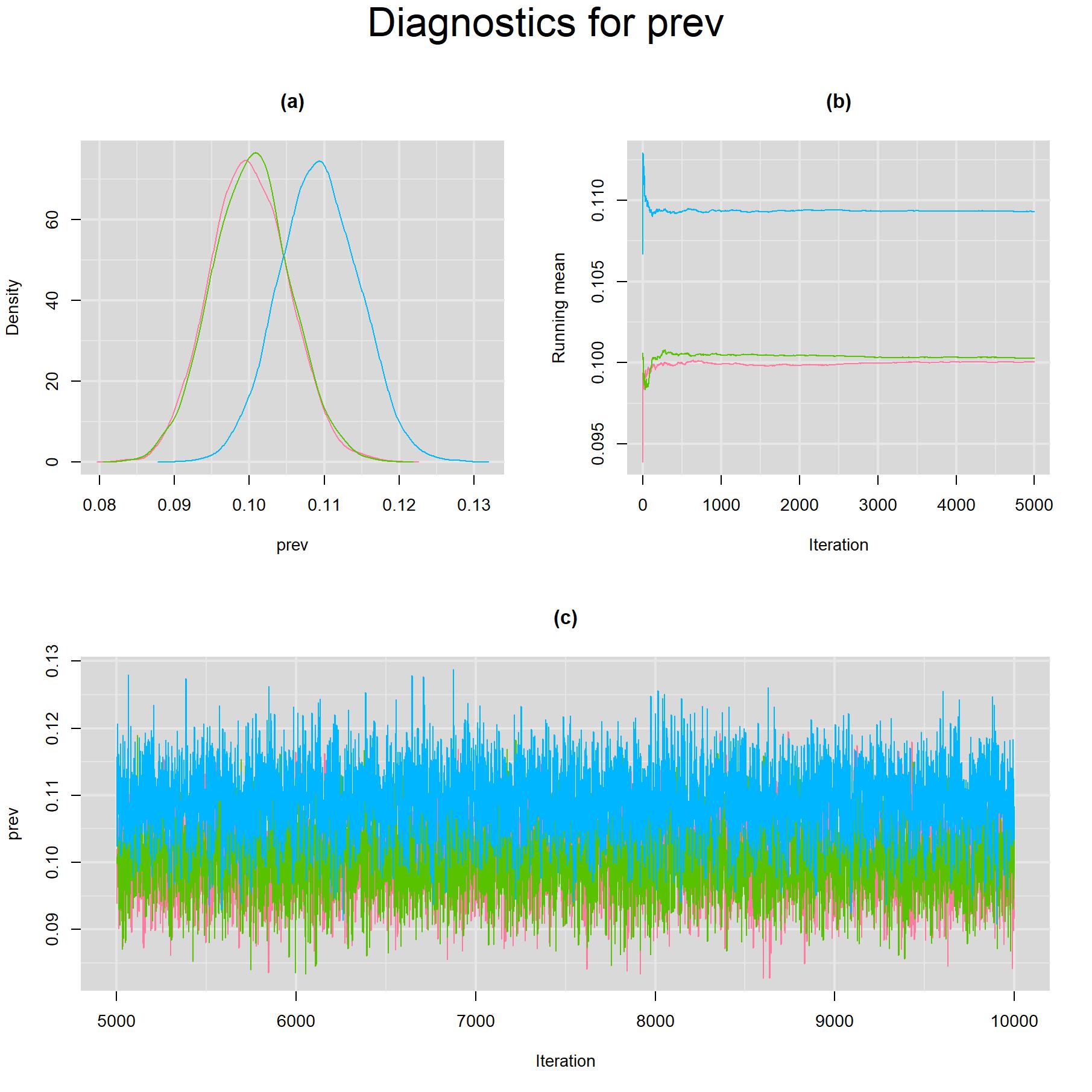
The plot above shows that two chains converged to the same solution (red and green chains) but the third did not (blue chain). This is not a problem of the MCMC algorithm, but rather a feature of the model used. A latent class model with K latent classes has the potential for K mirror solutions. In our case, the 3-latent class model could lead to 3 potential mirror-solutions. In the plot above, we actually reached 2 of the 3 possible mirror-solutions, but only one is clinically meaningful corresponding to the low prevalence estimate of roughly 10% (red and green chains). Providing a better selection of initial values for the blue chain could actually avoid the blue chain reaching an undesired mirror-solution.

Index Test

Sensitivity and Specificity with respect to viable C. trachomatis bacteria (D)

for(k in 1:4) {
  for(i in 1:2) {
    #  tiff(paste(parameters[i],"[",j,"].tiff",sep=""),width = 23, height = 23, units = "cm", res=200)
    par(oma=c(0,0,3,0))
    layout(matrix(c(1,2,3,3), 2, 2, byrow = TRUE))
    denplot(output, parms=c(paste(parameters[i],"[",k,"]",sep="")), auto.layout=FALSE, main="(a)", xlab=paste(parameters[i],"",sep=""), ylab="Density")
    rmeanplot(output, parms=c(paste(parameters[i],"[",k,"]",sep="")), auto.layout=FALSE, main="(b)")
    title(xlab="Iteration", ylab="Running mean")
    traplot(output, parms=c(paste(parameters[i],"[",k,"]",sep="")), auto.layout=FALSE, main="(c)")
    title(xlab="Iteration", ylab=paste(parameters[i],"[",k,"]",sep=""))
    mtext(paste("Diagnostics for ", parameters[i],"[",k,"]","",sep=""), side=3, line=1, outer=TRUE, cex=2)
    #  dev.off()
  }
}

Prevalence of viable C. trachomatis bacteria (D)

for(i in 7) {
  #jpeg(paste(result_folder,"/",parameters[i],".jpeg",sep=""),width = 23, height = 23, units = "cm", res=200)
  par(oma=c(0,0,3,0))
  layout(matrix(c(1,2,3,3), 2, 2, byrow = TRUE))
  denplot(output, parms=c(paste(parameters[i], sep="")), auto.layout=FALSE, main="(a)", xlab=paste(parameters[i],"",sep=""), ylab="Density")
  rmeanplot(output, parms=c(paste(parameters[i], sep="")), auto.layout=FALSE, main="(b)")
  title(xlab="Iteration", ylab="Running mean")
  traplot(output, parms=c(paste(parameters[i], sep="")), auto.layout=FALSE, main="(c)")
  title(xlab="Iteration", ylab=paste(parameters[i], sep=""))
  mtext(paste("Diagnostics for ", parameters[i], sep=""), side=3, line=1, outer=TRUE, cex=2)
  #dev.off()
}

Sensitivity and Specificity with respect to C. trachomatis DNA (l1)

for(k in 1:4) {
  for(i in 3:4) {
    #  tiff(paste(parameters[i],"[",j,"].tiff",sep=""),width = 23, height = 23, units = "cm", res=200)
    par(oma=c(0,0,3,0))
    layout(matrix(c(1,2,3,3), 2, 2, byrow = TRUE))
    denplot(output, parms=c(paste(parameters[i],"[",k,"]",sep="")), auto.layout=FALSE, main="(a)", xlab=paste(parameters[i],"",sep=""), ylab="Density")
    rmeanplot(output, parms=c(paste(parameters[i],"[",k,"]",sep="")), auto.layout=FALSE, main="(b)")
    title(xlab="Iteration", ylab="Running mean")
    traplot(output, parms=c(paste(parameters[i],"[",k,"]",sep="")), auto.layout=FALSE, main="(c)")
    title(xlab="Iteration", ylab=paste(parameters[i],"[",k,"]",sep=""))
    mtext(paste("Diagnostics for ", parameters[i],"[",k,"]","",sep=""), side=3, line=1, outer=TRUE, cex=2)
    #  dev.off()
  }
}

Prevalence of C. trachomatis DNA (l1)

for(i in 8) {
  #jpeg(paste(result_folder,"/",parameters[i],".jpeg",sep=""),width = 23, height = 23, units = "cm", res=200)
  par(oma=c(0,0,3,0))
  layout(matrix(c(1,2,3,3), 2, 2, byrow = TRUE))
  denplot(output, parms=c(paste(parameters[i], sep="")), auto.layout=FALSE, main="(a)", xlab=paste(parameters[i],"",sep=""), ylab="Density")
  rmeanplot(output, parms=c(paste(parameters[i], sep="")), auto.layout=FALSE, main="(b)")
  title(xlab="Iteration", ylab="Running mean")
  traplot(output, parms=c(paste(parameters[i], sep="")), auto.layout=FALSE, main="(c)")
  title(xlab="Iteration", ylab=paste(parameters[i], sep=""))
  mtext(paste("Diagnostics for ", parameters[i], sep=""), side=3, line=1, outer=TRUE, cex=2)
  #dev.off()
}

Latent class probabilities

for(k in 1:3) {
  for(i in 9) {
    #jpeg(paste(result_folder,"/",parameters[i],"[",k,"].jpeg",sep=""),width = 23, height = 23, units = "cm", res=200)
    par(oma=c(0,0,3,0))
    layout(matrix(c(1,2,3,3), 2, 2, byrow = TRUE))
    denplot(output, parms=c(paste(parameters[i],"[",k,"]",sep="")), auto.layout=FALSE, main="(a)", xlab=paste(parameters[i],"",sep=""), ylab="Density")
    rmeanplot(output, parms=c(paste(parameters[i],"[",k,"]",sep="")), auto.layout=FALSE, main="(b)")
    title(xlab="Iteration", ylab="Running mean")
    traplot(output, parms=c(paste(parameters[i],"[",k,"]",sep="")), auto.layout=FALSE, main="(c)")
    title(xlab="Iteration", ylab=paste(parameters[i],"[",k,"]",sep=""))
    mtext(paste("Diagnostics for ", parameters[i],"[",k,"]","",sep=""), side=3, line=1, outer=TRUE, cex=2)
    #dev.off()
  }
}

Random effects parameters

for(i in 5) { #POSITION OF THE PARAMETER IN THE "parameters" OBJECT
  for(k in 1:3){
    for(j in 1:4) { 
      #jpeg(paste(result_folder,"/",parameters[i],"[",k,",",j,"].jpeg",sep=""),width = 23, height = 23, units = "cm", res=200)
      par(oma=c(0,0,3,0))
      layout(matrix(c(1,2,3,3), 2, 2, byrow = TRUE))
      denplot(output, parms=c(paste(parameters[i],"[",k,",",j,"]",sep="")), auto.layout=FALSE, main="(a)", xlab=paste(parameters[i],"[",k,"]",sep=""), ylab="Density")
      rmeanplot(output, parms=c(paste(parameters[i],"[",k,",",j,"]",sep="")), auto.layout=FALSE, main="(b)")
      title(xlab="Iteration", ylab="Running mean")
      traplot(output, parms=c(paste(parameters[i],"[",k,",",j,"]",sep="")), auto.layout=FALSE, main="(c)")
      title(xlab="Iteration", ylab=paste(parameters[i],"[",k,",",j,"]",sep=""))
      mtext(paste("Diagnostics for ", parameters[i],"[",k,",",j,"]",sep=""), side=3, line=1, outer=TRUE, cex=2)
      #dev.off()
    }
  }
}

for(i in 6) {
  #jpeg(paste(result_folder,"/",parameters[i],".jpeg",sep=""),width = 23, height = 23, units = "cm", res=200)
  par(oma=c(0,0,3,0))
  layout(matrix(c(1,2,3,3), 2, 2, byrow = TRUE))
  denplot(output, parms=c(paste(parameters[i], sep="")), auto.layout=FALSE, main="(a)", xlab=paste(parameters[i],"",sep=""), ylab="Density")
  rmeanplot(output, parms=c(paste(parameters[i], sep="")), auto.layout=FALSE, main="(b)")
  title(xlab="Iteration", ylab="Running mean")
  traplot(output, parms=c(paste(parameters[i], sep="")), auto.layout=FALSE, main="(c)")
  title(xlab="Iteration", ylab=paste(parameters[i], sep=""))
  mtext(paste("Diagnostics for ", parameters[i], sep=""), side=3, line=1, outer=TRUE, cex=2)
  #dev.off()
}

Posterior Results

The MCMCsummary function will provide the following posterior statistics.

The mean,
The standard deviation (sd),
The median (50%)
The 95% credible interval (2.5% and 97.5%).

Convergence statistics are also provided.

Rhat is the Gelman-Rubin statistic (Gelman and Rubin (1992), Brooks and Gelman (1998)). It is enabled when 2 or more chains are generated. It evaluates MCMC convergence by comparing within- and between-chain variability for each model parameter. Rhat tends to 1 as convergence is approached.
n.eff is the effective sample size (Gelman et al. (2013)). Because the MCMC process causes the posterior draws to be correlated, the effective sample size is an estimate of the sample size required to achieve the same level of precision if that sample was a simple random sample. When draws are correlated, the effective sample size will generally be lower than the actual numbers of draws resulting in poor posterior estimates.

Because of the presence of mirror-solutions, we are only extracting the posterior samples from chain 1, which is one of the 2 chains that displayed clinically meaningful results for the prevalence of viable C. trachomatis bacteria in the plot seen above.

res = MCMCsummary(output[[1]], digits=4, Rhat=FALSE)
datatable(res, extensions = 'AutoFill')

References

Citation

Black, Marrazzo, CM., and DH. Martin. 2002. “Head-to-head multicenter comparison of dna probe and nucleic acid ampliﬁcation tests for Chlamydia trachomatis infection in women performed with an improved reference standard.” Journal of Clinical Microbiology, no. 40: 3757–63.

Brooks, S. P., and A Gelman. 1998. “General methods for monitoring convergence of iterative simulations.” Journal of Computational and Graphical Statistics, no. 7: 434–55.

Dendukuri, Hadgu, N., and L. Wang. 2009. “Modeling conditional dependence between diagnostic tests: a multiple latent variable model.” Stat Med, no. 28(3): 441–61.

Gelman, A, J. B. Carlin, H. S. Stern, D. B. Dunson, A Vehtari, and D. B. Rbin. 2013. “Bayesian Data Analysis.” Chapman & Hall/CRC Press, London, Third Edition.

Gelman, A, and D. B. Rubin. 1992. “Inference from iterative simulation using multiple sequences.” Statistical Sciences, no. 7: 457–72.

Citation

BibTeX citation:

@online{schiller2024,
  author = {Ian Schiller and Nandini Dendukuri},
  title = {Bayesian {3-LC} {Random} {Effects} {Model}},
  date = {2024-01-11},
  url = {https://www.nandinidendukuri.com/LCA/Bayesian_3-LC_Random_Effects_Models.html/},
  langid = {en}
}

For attribution, please cite this work as:

Ian Schiller, and Nandini Dendukuri. 2024. “Bayesian 3-LC Random Effects Model.” January 11, 2024. https://www.nandinidendukuri.com/LCA/Bayesian_3-LC_Random_Effects_Models.html/.

Introduction

Download rjags Script

Script Instructions

Suggested R Package

C.trachomatis Dataset

Bayesian Latent Class Random Effects Model

Prior Distributions

Initial Values

Compiling the model with rjags

Posterior Sampling

Convergence Diagnostic Plots

Index Test

Sensitivity and Specificity with respect to viable C. trachomatis bacteria (D)

Prevalence of viable C. trachomatis bacteria (D)

Sensitivity and Specificity with respect to C. trachomatis DNA (l1)

Prevalence of C. trachomatis DNA (l1)

Latent class probabilities

Random effects parameters

Posterior Results

References

Citation

Citation

Download `rjags` Script

Suggested `R Package`

Compiling the model with `rjags`