Bayesian 2-LC Random Effects Model

Authors

Ian Schiller

Nandini Dendukuri

Published

January 11, 2024

Introduction

This article is intended to give the reader basic instructions on how to run an rjags script to perform a Bayesian analysis of diagnostic test accuracy and disease prevalence in the absence of a perfect reference test with a 2-latent class random effects model (Dendukuri and Joseph (2001)). The script is implemented in R using the rjags package, which interfaces with the JAGS (Just Another Gibbs Sampler) software for Bayesian analysis.

The term “2-latent class” refers to the presence of two hidden or latent classes in the data - often referred to in diagnostic test accuracy research as target condition positive and target condition negative.

Random effects are incorporated into the model to account for conditional dependence between the observed diagnostic tests.

An example dataset is provided for the user to familiarize themself with the script. It is from a study conducted to estimate the prevalence of Strongyloides infection among a group of Cambodian refugees to Canada (Joseph and Coupal (1995)).

Download `rjags` Script

The full script, can be downloaded here.

Script Instructions

Suggested `R Package`

Below is a list of packages we recommend installing. Aside from rjags, which is mandatory, the other packages are optional when performing LC analysis. We do recommend them as they are used in the script. Be aware that some functionalities of the script may not work if you do not install every package listed below.

require(rjags)     # PACKAGE TO RUN THE jags MODEL. MANDATORY
require(MCMCvis)   # THIS PACKAGE CONTAINS THE MCMCsummary FUNCTION USED IN THIS SCRIPT
require(mcmcplots) # USED FOR THE CREATION OF THE CONVERGENCE PLOTS
require(DT)        # THIS LIBRARY ALLOWS A NICE DATA DISPLAY WITH THE SEARCH BAR OPTION.

Strongyloides Dataset

The Strongyloides dataset is taken from a study conducted to estimate the prevalence of Strongyloides infection among a group of Cambodian refugees to Canada). It includes 162 participants with results on 2 diagnostic tests. From a notation point of view, we suppose here that the Stool examination is the reference test and the Serology test is the index test.

n11 cell = Number of patients positive on both tests
n10 cell = Number of patients positivie on first test (index test) and negative on second test (reference test)
n01 cell = Number of patients negative on first test (index test) and positive on second test (reference test)
n00 cell = Number of patients negative on both tests

We recommend to save the Strongyloides dataset in a . txt extension file as Strongyloides.txt in the same folder as the script. The data can be uploaded with the read.table function. The data comprises a single row and 4 columns whose entries are the number of patients falling in each of the 4 categories defined above (n11, n10, n01, n00).

DATA <- read.table("Strongyloides.txt", header=TRUE)
datatable(DATA, extensions = 'AutoFill')#, options = list(autoFill = TRUE))

This data formatting is however not compatible with the model we will write below, as we need to express the data on an individual level and store it in a list we call dataList. The data that will be included in dataList are the sample size, noted N and the actual joint test results of each individual subject, noted y.

# Single patient result for the first (t1) and second (t2) test
t1 <- c(rep(1, DATA$n11), rep(1, DATA$n10), rep(0, DATA$n01), rep(0, DATA$n00) )
t2 <- c(rep(1, DATA$n11), rep(0, DATA$n10), rep(1, DATA$n01), rep(0, DATA$n00) )
# Joint test results for each patient
y <- cbind(t1, t2)
# Number of patients
N = dim(y)[1]

dataList <- list(y=y, N=N)

As seen below, the data y contains as many rows as there are subjects and both columns represent the subject’s test results.

datatable(y, extensions = 'AutoFill')#, options = list(autoFill = TRUE))

Bayesian Latent Class Random Effects Model

Implementing the Bayesian 2-latent class random effects model in rjags involves specifying the priors and likelihood. Markov Chain Monte Carlo (MCMC) methods, such as Gibbs sampling, are then employed to estimate the posterior distribution of the model parameters.

The rjags model is saved on the current directory (where your script and data should already be saved ideally) as model.txt. Below is the model following the JAGS syntax.

modelString =

"model {

for (i in 1:N) {

  #============
  # LIKELIHOOD 
  #============
  
    D1[i]~dbern(prev)
    D[i]<-D1[i]+1
    y[i,1]~dbern(p1[i,D[i]])
    y[i,2]~dbern(p2[i,D[i]])
    
    # Defining the sensitivity and specificity of each subject (with inclusion of random effects)
    r[i]~dnorm(0,1)
    s1[i]<-phi(a[1,1]+b.RE[1]*r[i])
    c1[i]<-phi(a[1,2]+b.RE[2]*r[i])
    s2[i]<-phi(a[2,1]+b.RE[1]*r[i])
    c2[i]<-phi(a[2,2]+b.RE[2]*r[i])
    
    # Conditional probability of a positive observation
    p1[i,2]<-s1[i]
    p1[i,1]<-1-c1[i]
    p2[i,2]<-s2[i]
    p2[i,1]<-1-c2[i]

}

#==================================================
# Prior distributions
#==================================================

prev~dbeta(1,1)
se[1]~dbeta(21.96,5.49)
sp[1]~dbeta(4.1,1.76) 
se[2]~dbeta(4.44,13.31)
sp[2]~dbeta(71.25,3.75)


a[1,1]<-probit(se[1])*sqrt(1+b.RE[1]*b.RE[1])
a[1,2]<-probit(sp[1])*sqrt(1+b.RE[1]*b.RE[1])
a[2,1]<-probit(se[2])*sqrt(1+b.RE[2]*b.RE[2])
a[2,2]<-probit(sp[2])*sqrt(1+b.RE[2]*b.RE[2])

b.RE[1]~dnorm(0,1)I(0,)
b.RE[2]~dnorm(0,1)I(0,)

}"

writeLines(modelString,con="model.txt")

Prior Distributions

The prior distributions used in the script are inspired from those provided in Dendukuri and Joseph (2001).

A Beta(1,1) prior distribution was used for the prevalence parameter which is equivalent to a Uniform(0,1) vague prior.

In a random effects model, prior distributions need to be placed on the a and b parameters as the sensitivity and specificity are functions of these parameters. This often turns out not to be straightforward. Also, expert opinions that are used to derive prior distributions are often expressed as the sensitivity and specificity of the tests. Therefore, in this script we provide Beta prior distributions for the sensitivity and specificity of both tests as explained in this blog article (Specifying prior distribution for diagnostic test accuracy in latent class model with random effects) and low information prior distributions on the b parameters. This induces a prior distribution on the a parameters.

For test 1 (index test =Serology test)

\(se[1] \sim Beta(21.96,5.49)\)
\(sp[1] \sim Beta(4.1,1.76)\)

For test 2 (reference test =Stool examination)

\(se[2] \sim Beta(4.44,13.31)\)
\(sp[2] \sim Beta(71.25,3.75)\)

Truncated normal prior distributions are used for the random effects parameters as followed

\(b.RE[1] \sim N(0,1)I(0,)\)
\(b.RE[2] \sim N(0,1)I(0,)\)

Initial Values

Initial values are needed as the starting point for estimating and updating parameters of the model in rjags. We strongly encourage the user to provide their own method of generating initial values rather than counting on rjags to generate them. Initial values can be provided in different ways in rjags. We propose one method below based on the creation of a home made function to randomly generate initial values based on the prior distributions. For more options on how to provide initial values, please see A guide on how to provide initial values in rjags

# Initial values

GenInits  = function(){
  
    se1 <- rbeta(1,21.96,5.49)
    sp1 <- rbeta(1,4.1,1.76) 
    se2 <- rbeta(1,4.44,13.31)
    sp2 <- rbeta(1,71.25,3.75)
    b1 <- abs(rnorm(1,0,1))
    b2 <- abs(rnorm(1,0,1))
    prev <- rbeta(1,1,1)
    
    se <- c(se1, se2)
    sp <- c(sp1, sp2)
    b.RE <- c(b1, b2)
   
    list(
      se = se,
      sp = sp,
      b.RE = b.RE,
      prev = prev,
      .RNG.name="base::Wichmann-Hill",
      .RNG.seed=321
    )

}

Below we use our created GenInits function to initialize 3 chains. ** We provide a Seed value for reproducibility : **

# Initial values
set.seed(123)
initsList = vector('list',3)
for(i in 1:3){
    initsList[[i]] = GenInits()
}

Compiling the model with `rjags`

We compile the model with the jags.model function.

# Compile the model
jagsModel = jags.model("model.txt",data=dataList,n.chains=3,n.adapt=0, inits=initsList)

Compiling model graph
   Resolving undeclared variables
   Allocating nodes
Graph information:
   Observed stochastic nodes: 324
   Unobserved stochastic nodes: 331
   Total graph size: 3110

Initializing model

Posterior Sampling

The posterior samples for the parameters of the model are obtained by running more than one independent chain having its own starting values to assess convergence of the MCMC algorithm. Here in the script, we elected to run 3 separate chains.

The posterior sampling step is in fact a 2-part step.

First we discard a certain number of iterations with the update function. This step is often referred to as the Burn-in step and is needed to prevent the posterior samples including subset of samples obtained while the algorithm had not yet converged. Here, we elected to discard 5,000 iterations.
Then we use the coda.samples function to sample another 5,000 iterations from the posterior distribution. The posterior sample assembled is stored in the output object.

Generally, the number of burn-in and sampling iterations needed will depend on the complexity of the model, the prior distribution as well as the quality of the initial values.

#jagsModel$state(internal=FALSE)

# Burn-in iterations 
update(jagsModel,n.iter=5000)
# Parameters to be monitored
parameters = c( "se","sp", "a", "b.RE", "prev")

# Posterior samples
posterior_results = coda.samples(jagsModel,variable.names=parameters,n.iter=5000)
output = posterior_results

Posterior Results

The MCMCsummary function will provide the following posterior statistics.

The mean,
The standard deviation (sd),
The median (50%)
The 95% credible interval (2.5% and 97.5%).

Convergence statistics are also provided.

Rhat is the Gelman-Rubin statistic (Gelman and Rubin (1992), Brooks and Gelman (1998)). It is enabled when 2 or more chains are generated. It evaluates MCMC convergence by comparing within- and between-chain variability for each model parameter. Rhat tends to 1 as convergence is approached.
n.eff is the effective sample size (Gelman et al. (2013)). Because the MCMC process causes the posterior draws to be correlated, the effective sample size is an estimate of the sample size required to achieve the same level of precision if that sample was a simple random sample. When draws are correlated, the effective sample size will generally be lower than the actual numbers of draws resulting in poor posterior estimates.

res = MCMCsummary(output, digits=4)
datatable(res, extensions = 'AutoFill')

Convergence Diagnostic Plots

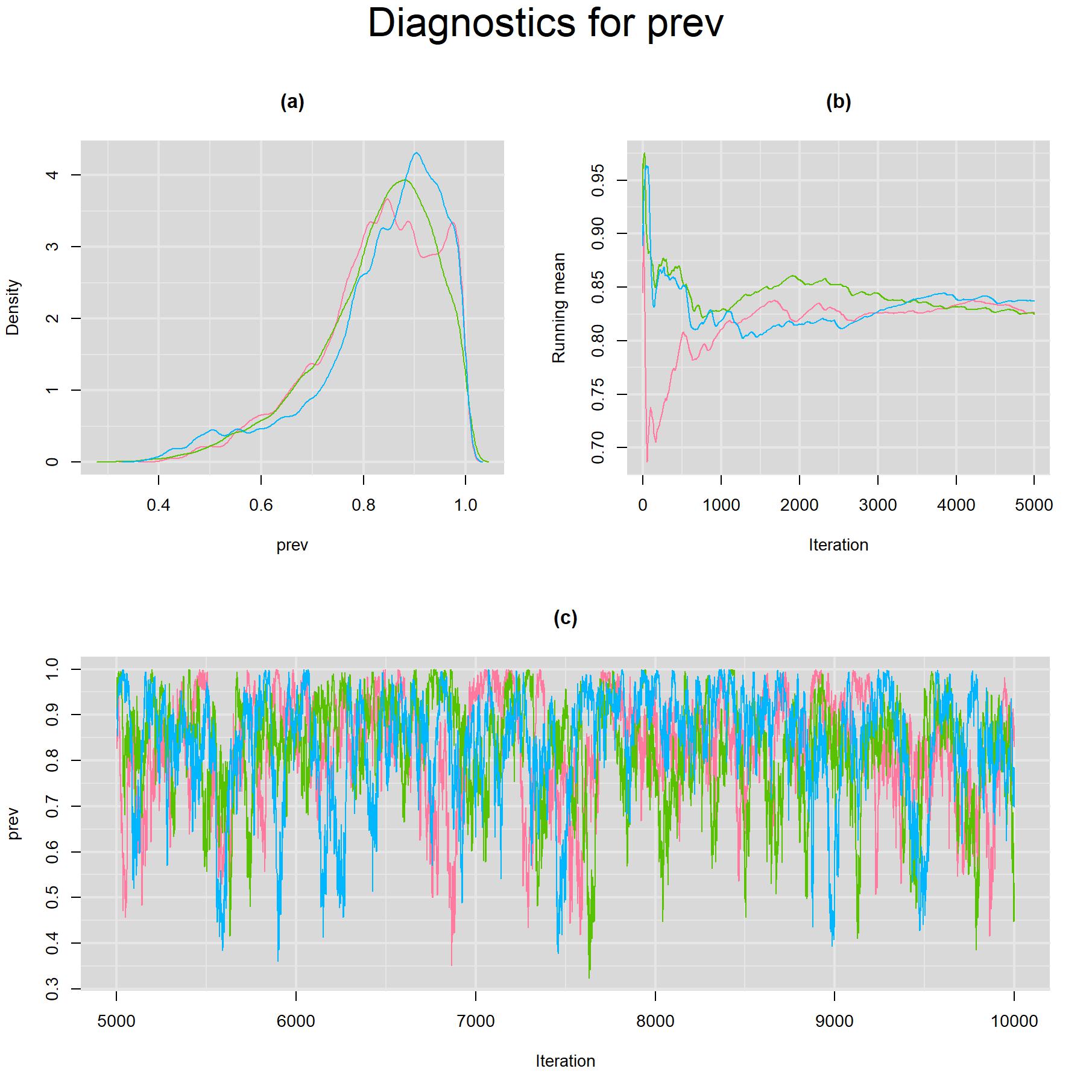
Visual inspection of convergence for key parameters can be studied using different tools. We opted to write our own code as it gives us more flexibility and control on what we want to display. For a given parameter, panel (a) shows posterior density plot; (b) the running posterior mean value; and (c) the history plot. Each chain is identified by a different color. Similar behavior from all 3 chains would suggest the algorithm has converged. For example, here is the 3-panel plot for the prevalence parameter.

Index Test SEROLOGY TEST

Sensitivity and Specificity

for(k in 1) {
  for(i in 1:2) {
    #  tiff(paste(parameters[i],"[",j,"].tiff",sep=""),width = 23, height = 23, units = "cm", res=200)
    par(oma=c(0,0,3,0))
    layout(matrix(c(1,2,3,3), 2, 2, byrow = TRUE))
    denplot(output, parms=c(paste(parameters[i],"[",k,"]",sep="")), auto.layout=FALSE, main="(a)", xlab=paste(parameters[i],"",sep=""), ylab="Density")
    rmeanplot(output, parms=c(paste(parameters[i],"[",k,"]",sep="")), auto.layout=FALSE, main="(b)")
    title(xlab="Iteration", ylab="Running mean")
    traplot(output, parms=c(paste(parameters[i],"[",k,"]",sep="")), auto.layout=FALSE, main="(c)")
    title(xlab="Iteration", ylab=paste(parameters[i],"[",k,"]",sep=""))
    mtext(paste("Diagnostics for ", parameters[i],"[",k,"]","",sep=""), side=3, line=1, outer=TRUE, cex=2)
    #  dev.off()
  }
}

# Plots to check convergence for parameters shared across studies:

for(i in c(4)) { #POSITION OF THE PARAMETER IN THE "parameters" OBJECT
  for(k in 1){
    #  tiff(paste(parameters[i],"[",k,"].tiff",sep=""),width = 23, height = 23, units = "cm", res=200)
    par(oma=c(0,0,3,0))
    layout(matrix(c(1,2,3,3), 2, 2, byrow = TRUE))
    denplot(output, parms=c(paste(parameters[i],"[",k,"]",sep="")), auto.layout=FALSE, main="(a)", xlab=paste(parameters[i],"[",k,"]",sep=""), ylab="Density")
    rmeanplot(output, parms=c(paste(parameters[i],"[",k,"]",sep="")), auto.layout=FALSE, main="(b)")
    title(xlab="Iteration", ylab="Running mean")
    traplot(output, parms=c(paste(parameters[i],"[",k,"]",sep="")), auto.layout=FALSE, main="(c)")
    title(xlab="Iteration", ylab=paste(parameters[i],"[",k,"]",sep=""))
    mtext(paste("Diagnostics for ", parameters[i],"[",k,"]",sep=""), side=3, line=1, outer=TRUE, cex=2)
    #  dev.off()
  }
}

# Plots to check convergence for parameters shared across studies:

for(i in c(3)) { #POSITION OF THE PARAMETER IN THE "parameters" OBJECT
  for(k in 1){
    for(j in 1:2) { 
      #  tiff(paste(parameters[i],"[",k,"].tiff",sep=""),width = 23, height = 23, units = "cm", res=200)
      par(oma=c(0,0,3,0))
      layout(matrix(c(1,2,3,3), 2, 2, byrow = TRUE))
      denplot(output, parms=c(paste(parameters[i],"[",k,",",j,"]",sep="")), auto.layout=FALSE, main="(a)", xlab=paste(parameters[i],"[",k,"]",sep=""), ylab="Density")
      rmeanplot(output, parms=c(paste(parameters[i],"[",k,",",j,"]",sep="")), auto.layout=FALSE, main="(b)")
      title(xlab="Iteration", ylab="Running mean")
      traplot(output, parms=c(paste(parameters[i],"[",k,",",j,"]",sep="")), auto.layout=FALSE, main="(c)")
      title(xlab="Iteration", ylab=paste(parameters[i],"[",k,",",j,"]",sep=""))
      mtext(paste("Diagnostics for ", parameters[i],"[",k,",",j,"]",sep=""), side=3, line=1, outer=TRUE, cex=2)
      #  dev.off()
    }
  }
}

Reference Test STOOL EXAMINATION

Sensitivity and Specificity

for(k in 2) {
  for(i in 1:2) {
    #  tiff(paste(parameters[i],"[",j,"].tiff",sep=""),width = 23, height = 23, units = "cm", res=200)
    par(oma=c(0,0,3,0))
    layout(matrix(c(1,2,3,3), 2, 2, byrow = TRUE))
    denplot(output, parms=c(paste(parameters[i],"[",k,"]",sep="")), auto.layout=FALSE, main="(a)", xlab=paste(parameters[i],"",sep=""), ylab="Density")
    rmeanplot(output, parms=c(paste(parameters[i],"[",k,"]",sep="")), auto.layout=FALSE, main="(b)")
    title(xlab="Iteration", ylab="Running mean")
    traplot(output, parms=c(paste(parameters[i],"[",k,"]",sep="")), auto.layout=FALSE, main="(c)")
    title(xlab="Iteration", ylab=paste(parameters[i],"[",k,"]",sep=""))
    mtext(paste("Diagnostics for ", parameters[i],"[",k,"]","",sep=""), side=3, line=1, outer=TRUE, cex=2)
    #  dev.off()
  }
}

# Plots to check convergence for parameters shared across studies:

for(i in c(4)) { #POSITION OF THE PARAMETER IN THE "parameters" OBJECT
  for(k in 2){
    #  tiff(paste(parameters[i],"[",k,"].tiff",sep=""),width = 23, height = 23, units = "cm", res=200)
    par(oma=c(0,0,3,0))
    layout(matrix(c(1,2,3,3), 2, 2, byrow = TRUE))
    denplot(output, parms=c(paste(parameters[i],"[",k,"]",sep="")), auto.layout=FALSE, main="(a)", xlab=paste(parameters[i],"[",k,"]",sep=""), ylab="Density")
    rmeanplot(output, parms=c(paste(parameters[i],"[",k,"]",sep="")), auto.layout=FALSE, main="(b)")
    title(xlab="Iteration", ylab="Running mean")
    traplot(output, parms=c(paste(parameters[i],"[",k,"]",sep="")), auto.layout=FALSE, main="(c)")
    title(xlab="Iteration", ylab=paste(parameters[i],"[",k,"]",sep=""))
    mtext(paste("Diagnostics for ", parameters[i],"[",k,"]",sep=""), side=3, line=1, outer=TRUE, cex=2)
    #  dev.off()
  }
}

# Plots to check convergence for parameters shared across studies:

for(i in c(3)) { #POSITION OF THE PARAMETER IN THE "parameters" OBJECT
  for(k in 2){
    for(j in 1:2) { 
      #  tiff(paste(parameters[i],"[",k,"].tiff",sep=""),width = 23, height = 23, units = "cm", res=200)
      par(oma=c(0,0,3,0))
      layout(matrix(c(1,2,3,3), 2, 2, byrow = TRUE))
      denplot(output, parms=c(paste(parameters[i],"[",k,",",j,"]",sep="")), auto.layout=FALSE, main="(a)", xlab=paste(parameters[i],"[",k,"]",sep=""), ylab="Density")
      rmeanplot(output, parms=c(paste(parameters[i],"[",k,",",j,"]",sep="")), auto.layout=FALSE, main="(b)")
      title(xlab="Iteration", ylab="Running mean")
      traplot(output, parms=c(paste(parameters[i],"[",k,",",j,"]",sep="")), auto.layout=FALSE, main="(c)")
      title(xlab="Iteration", ylab=paste(parameters[i],"[",k,",",j,"]",sep=""))
      mtext(paste("Diagnostics for ", parameters[i],"[",k,",",j,"]",sep=""), side=3, line=1, outer=TRUE, cex=2)
      #  dev.off()
    }
  }
}

Prevalence

for(i in 5) {
  # tiff(paste(parameters[i],".tiff",sep=""),width = 23, height = 23, units = "cm", res=200)
  par(oma=c(0,0,3,0))
  layout(matrix(c(1,2,3,3), 2, 2, byrow = TRUE))
  denplot(output, parms=c(paste(parameters[i], sep="")), auto.layout=FALSE, main="(a)", xlab=paste(parameters[i],"",sep=""), ylab="Density")
  rmeanplot(output, parms=c(paste(parameters[i], sep="")), auto.layout=FALSE, main="(b)")
  title(xlab="Iteration", ylab="Running mean")
  traplot(output, parms=c(paste(parameters[i], sep="")), auto.layout=FALSE, main="(c)")
  title(xlab="Iteration", ylab=paste(parameters[i], sep=""))
  mtext(paste("Diagnostics for ", parameters[i], sep=""), side=3, line=1, outer=TRUE, cex=2)
  # dev.off()
}

References

Brooks, S. P., and A Gelman. 1998. “General methods for monitoring convergence of iterative simulations.” Journal of Computational and Graphical Statistics, no. 7: 434–55.

Dendukuri, Nandini, and Lawrence Joseph. 2001. “Bayesian approaches to modeling the conditional dependence between multiple diagnostic tests.” Biometrics, no. March: 158–67. http://www.jstor.org/stable/2676854.

Gelman, A, J. B. Carlin, H. S. Stern, D. B. Dunson, A Vehtari, and D. B. Rbin. 2013. “Bayesian Data Analysis.” Chapman & Hall/CRC Press, London, Third Edition.

Gelman, A, and D. B. Rubin. 1992. “Inference from iterative simulation using multiple sequences.” Statistical Sciences, no. 7: 457–72.

Joseph, Gyorkos, L., and L. Coupal. 1995. “Bayesian estimation of disease prevalence and the parameters of diagnostic tests in the absence of a gold standard.” American Journal of Epidemiology, no. 141: 263–72.

Citation

BibTeX citation:

@online{schiller2024,
  author = {Ian Schiller and Nandini Dendukuri},
  title = {Bayesian {2-LC} {Random} {Effects} {Model}},
  date = {2024-01-11},
  url = {https://www.nandinidendukuri.com/LCA/Bayesian_2-LC_Random_Effects_Models.html/},
  langid = {en}
}

For attribution, please cite this work as:

Ian Schiller, and Nandini Dendukuri. 2024. “Bayesian 2-LC Random Effects Model.” January 11, 2024. https://www.nandinidendukuri.com/LCA/Bayesian_2-LC_Random_Effects_Models.html/.

Introduction

Download rjags Script

Script Instructions

Suggested R Package

Strongyloides Dataset

Bayesian Latent Class Random Effects Model

Prior Distributions

Initial Values

Compiling the model with rjags

Posterior Sampling

Posterior Results

Convergence Diagnostic Plots

Index Test SEROLOGY TEST

Sensitivity and Specificity

Reference Test STOOL EXAMINATION

Sensitivity and Specificity

Prevalence

References

Citation

Download `rjags` Script

Suggested `R Package`

Compiling the model with `rjags`