–
Background
About two decades ago we described Bayesian inference for a latent class model with random effects, motivated by an application to estimate diagnostic accuracy and disease prevalence in the absence of a perfect reference test (Dendukuri and Joseph 2001). The random effects served to model conditional dependence between imperfect diagnostic tests, i.e. to model the possibility that the imperfect tests are jointly false positive or false negative. The form of the prior distributions we used at that time for the sensitivities and specificities was unnecessarily complicated, relying on a bisectional search. A more straightforward approach is described in the current article. Though the text below refers to the sensitivity, it applies equally to the specificity.
Model
The sensitivity of the ith individual is expressed as \(\Phi(a+br_i)\) where \(a\) and \(b\) are unknown parameters, \(r_i\) is a random effect following a standard normal distribution \(r_i \sim N(0,1)\) and \(\Phi\) denotes the cumulative probability of the standard normal distribution. For simplicity the subscript \(i\) of the random effect is suppressed and it is written as \(r\) in the rest of this document. It can be shown that the marginal (or average) sensitivity, across all values of \(r\), is \(S=\Phi(\frac{a}{\sqrt{1+b^2}})\).
Visualizing the distribution of sensitivity
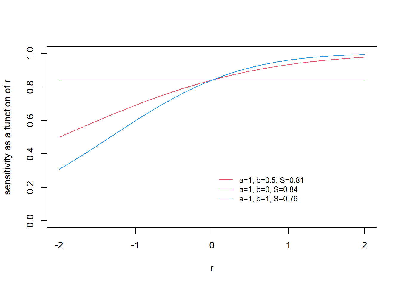
Consider the case when \(a=1\) and \(b=0.5\). The relation between the sensitivity of the ith individual and \(r\) is illustrated by the red line in the graph below:
In this case the marginal sensitivity \(S = \Phi(\frac{1}{\sqrt{1+0.5^2}})\) = 0.81. We can see from the plot above that individual sensitivities range from roughly 0.5 to 0.95. The sensitivity for an individual with \(r\)=0 is \(\Phi(1)\)=0.84 which is close to the marginal sensitivity.
If \(b\) were 0 then the sensitivity would be the same for all subjects, \(S=0.84\) (green line). When \(b\) increases to 1 (blue line) the the variation in sensitivity across individuals increases, though the marginal sensitivity (\(S\)) does not change as much. Thus the plot above shows that \(a\) has a greater influence on the marginal sensitivity while \(b\) exerts influence on the range of sensitivity across individuals.
Prior information
Prior information is typically available on the marginal sensitivity (\(S\)). However, the model likelihood is expressed in terms of the individual sensitivities which are functions of both \(a\) and \(b\) and we need to specify a prior distribution for each of \(a\) and \(b\). In other words, we have to translate the prior information on a single variable (\(S\)) into prior distributions on two parameters \(a\) and \(b\).
Translating prior information into prior distributions
Keeping in mind that \(b\) has a lesser influence on the marginal sensitivity, we can assign it a weakly informative prior distribution, e.g. \(b \sim Uniform(0,3)\). Instead of providing a prior distribution for \(a\), we can provide a prior distribution for \(S\) and express \(a\) as a function of the marginal sensitivity and \(b\), i.e. \(a=\Phi^{-1}(S)\sqrt(1+b^2)\).
Example
We now apply the ideas above to the Strongyloides infection example reported in the paper by Dendukuri and Joseph. The equal-tailed 95% prior credible interval over the marginal sensitivity of microscopy was (7%, 47%). In the absence of any prior information on the individual sensitivities we could assume a very wide range from (0%, 100%). This is equivalent to saying that there are some individuals in whom the test has 0% sensitivity and at the other extreme there are patients in whom it has a 100% sensitivity. It is possible that such a gradation is created by the severity of infection. Patients with a mild infection may have a very low count of the parasite that is not detectable by microscopy and those with a severe infection and correspondingly high count are always detected.
We first look at the case when \(b\) follows a Uniform(0,3) distribution. The prior distributions of \(a\) and \(b\) can be sampled from using the following R code
b=runif(1000,0,3)
S=rbeta(1000,4.44,13.31)
a=qnorm(S)*sqrt(1+b*b)
r=rnorm(1000,0,1)
S_i=pnorm(a+b*r)
The figure below illustrates the histograms of \(a\), \(b\), \(S\) and \(S_i\) (the individual sensitivity). It is interesting to note that \(a\) is more likely to be negative and the value of \(S_i\) is more likely to be 0, reflecting the low sensitivity of the test:
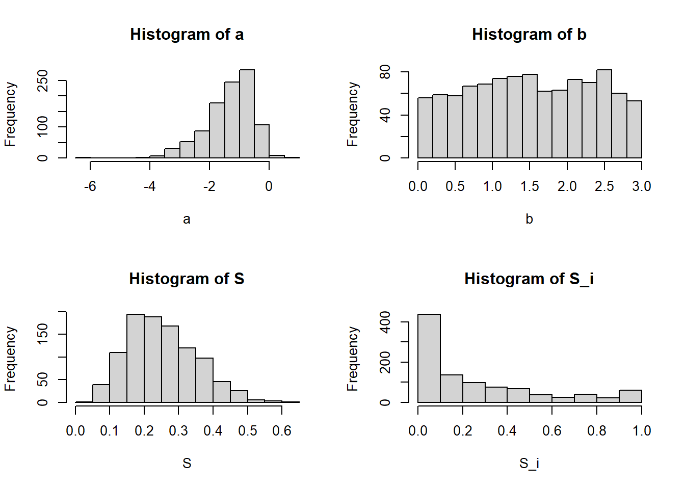
A look at the mean and quantiles of \(S\) and \(S_i\) (see below) helps to see that the mean of \(S\) and \(S_i\) are similar, while the median of \(S_i\) is lower than the median of \(S\):
round(quantile(S,c(0.025,0.5,0.975)),2) 2.5% 50% 97.5%
0.09 0.24 0.47 round(quantile(S_i,c(0.025,0.5,0.975)),2) 2.5% 50% 97.5%
0.00 0.15 0.99 round(mean(S),2)[1] 0.25round(mean(S_i),2)[1] 0.26The figures below illustrates the consequences of using \(b \sim Uniform(0,5)\) prior instead:
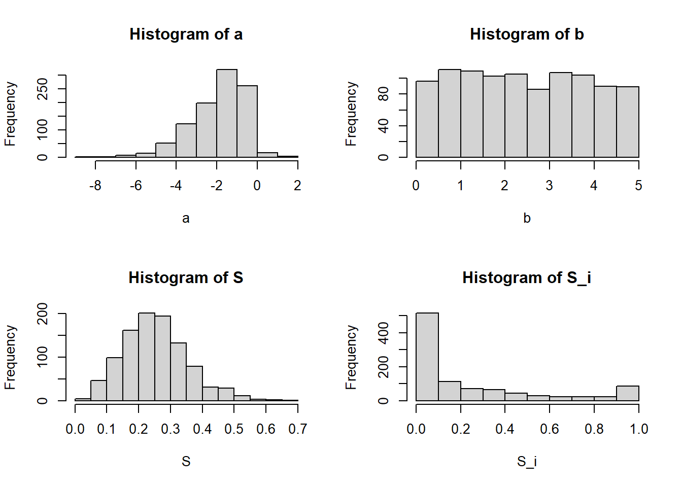
Once again, the mean values of \(S\) and \(S_i\) are similar. However, the median value of \(S_i\) is now even lower.
round(quantile(S,c(0.025,0.5,0.975)),2) 2.5% 50% 97.5%
0.08 0.25 0.48 round(quantile(S_i,c(0.025,0.5,0.975)),2) 2.5% 50% 97.5%
0.00 0.09 1.00 round(mean(S),2)[1] 0.25round(mean(S_i),2)[1] 0.24Finally, here is an illustration of the case when we have a non-informative, Uniform(0,1) prior over \(S\):
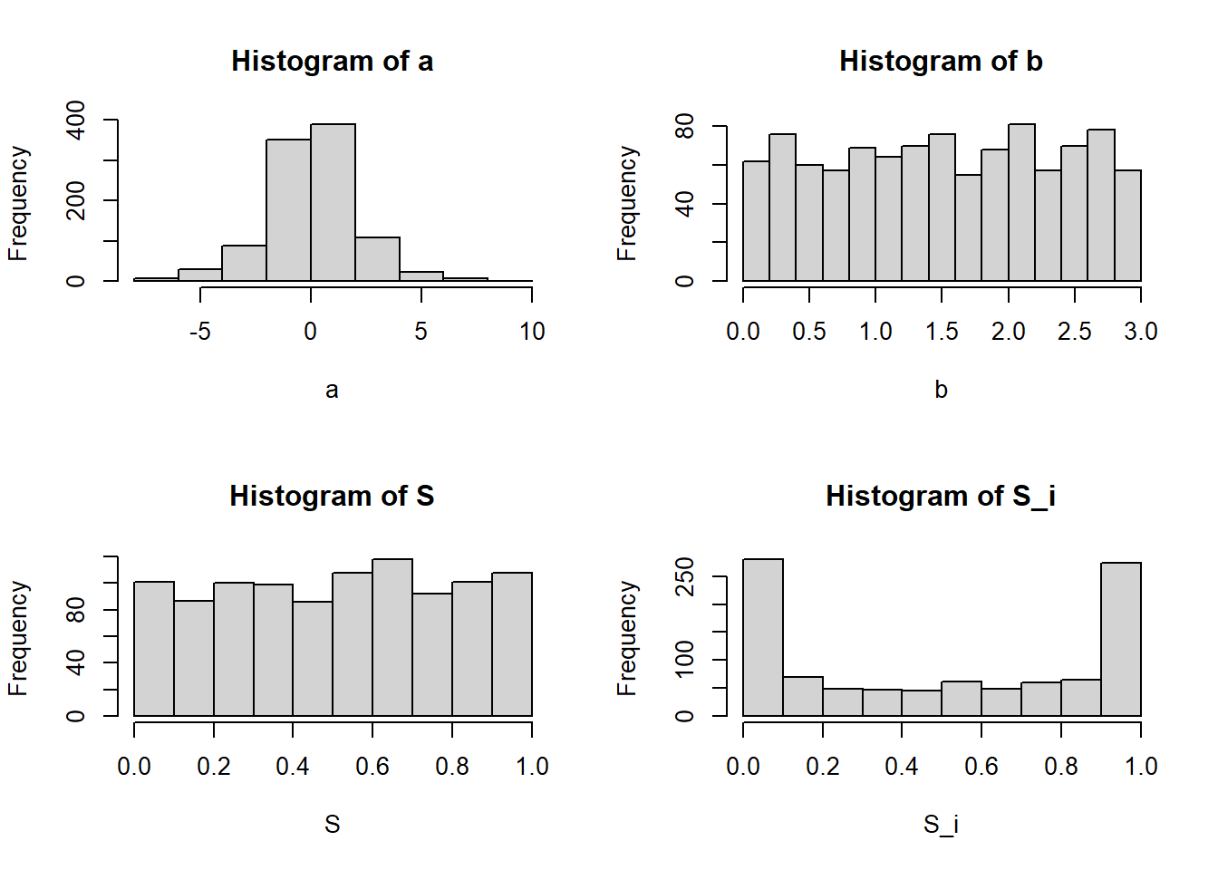
round(quantile(S,c(0.025,0.5,0.975)),2) 2.5% 50% 97.5%
0.02 0.52 0.98 round(quantile(S_i,c(0.025,0.5,0.975)),2) 2.5% 50% 97.5%
0.00 0.51 1.00 round(mean(S),2)[1] 0.51round(mean(S_i),2)[1] 0.5Summary
The approach described above is easier to implement. It has the additional advantage of ensuring the prior distribution on the marginal sensitivity \(S\) is the same as in a fixed effects latent class model. An rjags program to implement the revised prior distribution for the Strongyloides infection data can be found here. It is interesting to note that the posterior quantiles for the sensitivities, specificities and prevalence from the random effects model are now more similar to those obtained with the fixed effects model.
References
Dendukuri, Nandini, and Lawrence Joseph. 2001. “Bayesian approaches to modeling the conditional dependence between multiple diagnostic tests.” Biometrics, no. March: 158–67. http://www.jstor.org/stable/2676854.
Citation
BibTeX citation:
@online{dendukuri2022,
  author = {Nandini Dendukuri},
  title = {Specifying Prior Distribution for Diagnostic Test Accuracy in
    Latent Class Model with Random Effects},
  date = {2022-07-30},
  url = {https://www.nandinidendukuri.com/blogposts/2022-07-30-lca-remodel-prior/},
  langid = {en}
}
For attribution, please cite this work as:
Nandini Dendukuri. 2022. “Specifying Prior Distribution for
Diagnostic Test Accuracy in Latent Class Model with Random
Effects.” July 30, 2022. https://www.nandinidendukuri.com/blogposts/2022-07-30-lca-remodel-prior/.