OVERVIEW
Many researchers who wish to carry out diagnostic accuracy meta-analysis are not familiar with rjags. To address this we developed a Shiny app that is available on the net here. The programs behind this are the ones described in our previous blogs articles illustrating Rjags programs for diagnostic meta-analysis model (Bivariate model and Bivariate latent class model).
This blog article is intended to serve as a guide for the usage of the R Shiny app that implement the models discussed in the blog articles mentioned above. The main goal will be to describe the various options in the app via applied examples. The interested reader can learn more about the statistical theory in Dendukuri et al[-@Dendukuri2012].
The R Shiny app provides options to perform both Bayesian Bivariate meta-analysis and latent class meta-analysis.
MOTIVATING EXAMPLE AND DATA
For our motivating example we will use the data from a systematic review of studies evaluating the accuracy of GeneXpertTM (Xpert) test for tuberculosis (TB) meningitis (index test) and culture (reference test) for 29 studies (Kohli et al[-@Kohli2018]). Each study provides a two-by-two table of the form
| reference_test_positive | Reference_test_negative | |
|---|---|---|
| Index test positive | tp | fp |
| Index test negative | fn | tn |
where:
tpis the number of individuals who tested positive on both Xpert and culture testsfpis the number of individuals who tested positive on Xpert and negative on culture testfnis the number of individuals who tested negative on Xpert and positive on culture testtnis the number of individuals who tested negative on both Xpert and culture tests
We will explain later how to correctly supply the data into the app. Let’s first look at the 4 tab menus of the Shiny app.
Through this blog article, we will walk you through the 4 tab menus;
HomeManualBayesian Bivariate Meta-AnalysisLatent-Class Meta-Analysis
and we will explore features and options of each of them, starting with the Home tab menu.
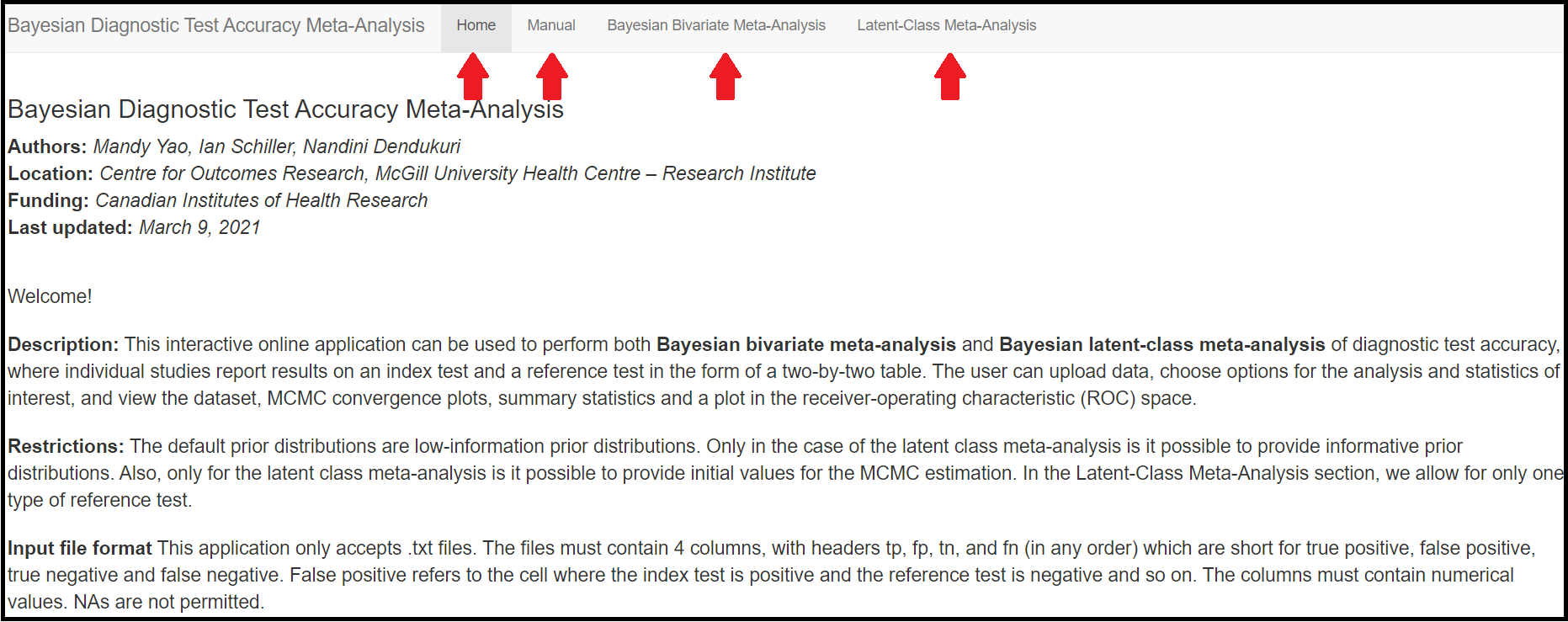
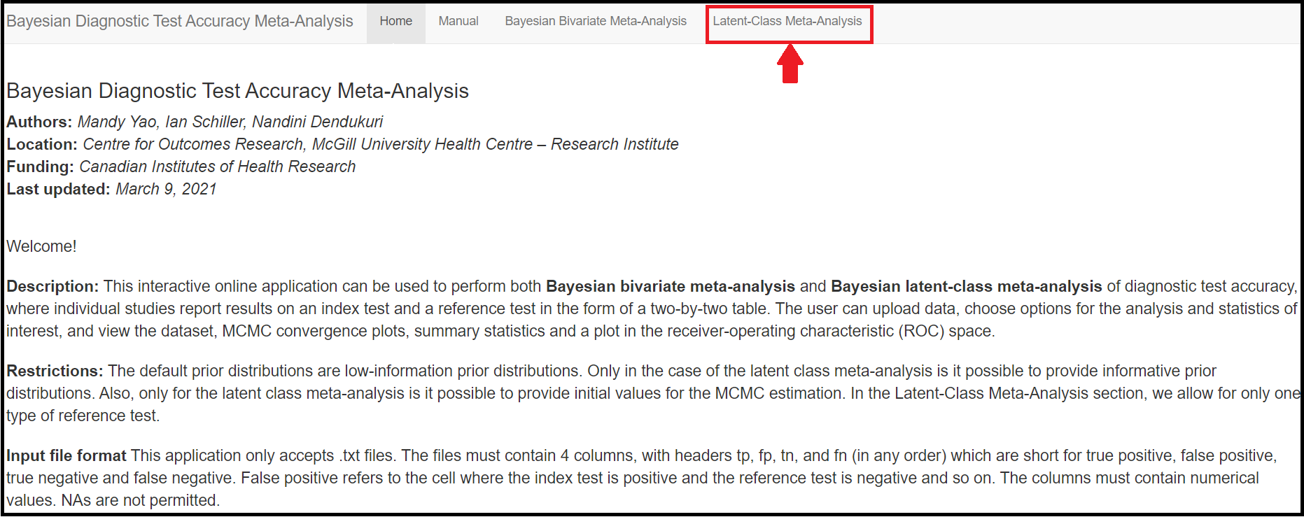
HOME
The Home tab menu gives a brief presentation of the app’s functionalities. It lists the restrictions of the app regarding the prior distributions used in the models or the initial values, as well as references to papers describing, among others, the theoretical models this app is based on.
It also details how the app expects the user to organize the data to be imported in the app at a later step. Basically, the data must be stored into a .txt file with 4 columns. The 4 column’s headers must be spelled exactly as tp , fp , fn and tn who were defined earlier in the OVERVIEW section, but the order in which the columns are presented in the file does not matter. Missing values or NA values are not supported. For example, the file Xpert_Data below would be a well defined .txt file to load into the app (we will see in a later section how to load the data in the app).
tp <- c(7, 6, 2, 5, 0, 1, 4, 3, 3, 1, 7, 35, 103, 1, 2, 22, 6, 25, 27, 15, 5, 2, 2, 11, 2, 0, 8, 3, 1)
fp <- c(5, 4, 0, 0, 0, 0, 6, 0, 3, 0, 0, 5, 6, 1, 0, 1, 1, 3, 11, 3, 9, 3, 0, 2, 4, 0, 2, 0, 2)
fn <- c(5, 4, 0, 1, 2, 0, 8, 1, 1, 0, 0, 1, 18, 2, 0, 5, 0, 20, 25, 7, 10, 1, 1, 2, 2, 3, 5, 0, 0)
tn <- c(63, 115, 2, 44, 132, 4, 83, 250, 67, 14, 150, 119, 252, 107, 8, 31, 148, 687, 204, 205, 115, 53, 4, 118, 22, 16, 186, 28, 43)
cell <- cbind(tp, fp, fn, tn)
n <- length(tp)  #  Number of studies
write("tp fp fn tn","Xpert_Data.txt")
for (j in 1:n) write(cell[j,],"Xpert_Data.txt",append=T)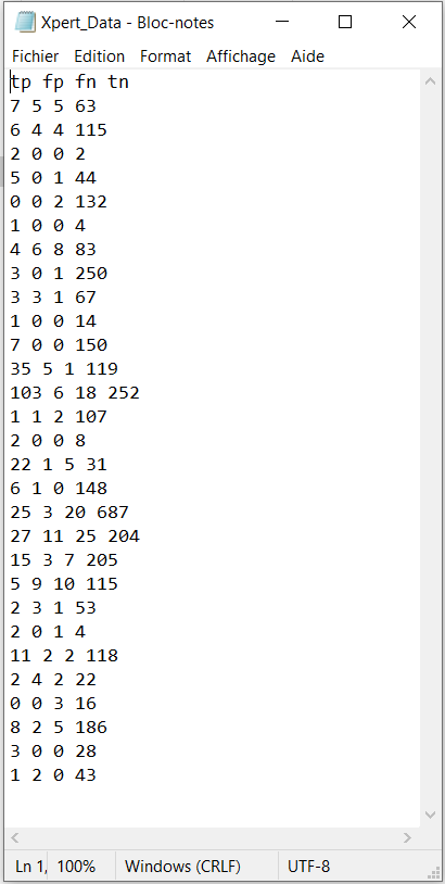
The user must note that when loading the data in the app, if the headers are not correctly spelled, if the number of columns differs from 4, if there are missing values or NA values in the file, then the Shiny App will fail and a Disconnected from the server error message like the one below will be displayed instead.

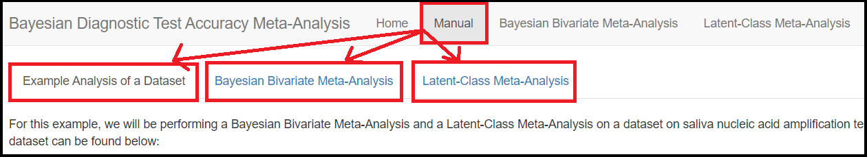
MANUAL
The MANUAL tab menu gives some basic guidelines on how to use the app features. It splits itself into 3 sub tab menus
Example Analysis of Dataset: Which gives a brief overview on how to prepare the data file to be loaded into the app.Bayesian Bivariate Meta-Analysis: how-to guide on how to use the app to model Bivariate meta-analysis.Latent-Class Meta-Analysis: how-to guide on how to use the app to model latent class meta-analysis.
BAYESIAN BIVARIATE MODEL
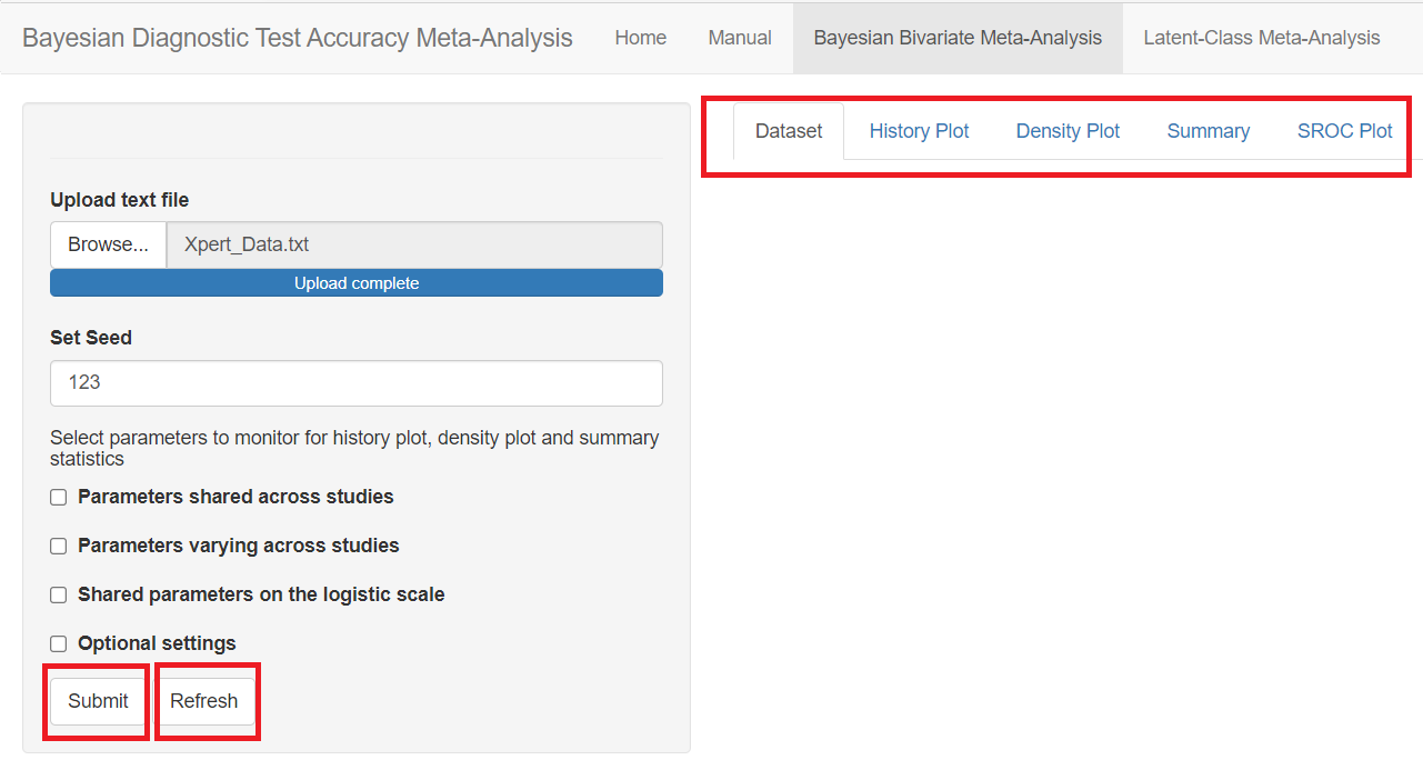
The Bayesian Bivariate Meta-Analysis is the tab menu that must be selected in order to perform a Bayesian bivariate meta-analysis. In this section, we will guide the user step by step to analyse the Xpert data presented in the MOTIVATING EXAMPLE AND DATA section in order to estimate Xpert’s accuracy under the assumption that culture is a perfect reference test.
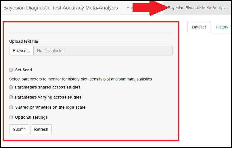
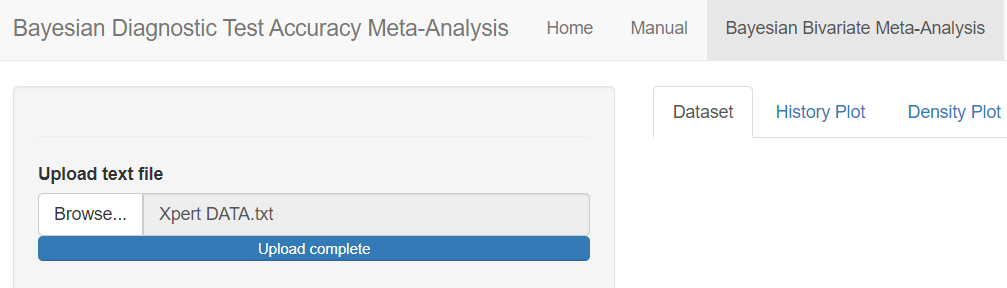
LOADING THE DATA
In the red rectangle of the screen shot above, uploading the text file that contains the data is the only feature that is mandatory before pressing the submit button. This is done by browsing your folders in order to load the data. Once done, an uploading bar will fill up and let you know that your data has been successfully loaded. Note that if there is a problem with the way you provided your data (missing values for instance), it is not until you press the submit button that the app will return the Disconnected from the server error message.
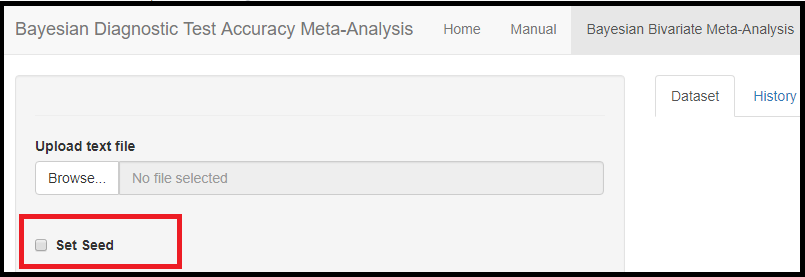
RANDOM SEED
The Set Seed feature is used to set the random number generator (RNG) state for random number generation in R. The default setting is to let the app randomly generates the RNG state. By checking the box next to Set Seed, the user can set up the RNG state for reproducibility of the results by entering a postive integer value. A value of 123 is suggested, but can be changed by the user.
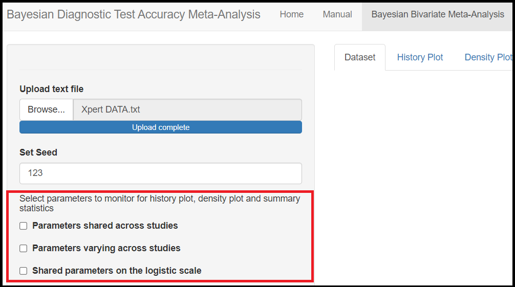
MONITORING PARAMETERS
Below the seed option are check-box options to select the various parameters of the model. Although it is specified to select parameters you want to monitor, there is actually no need to do that as the model will monitor every parameters of the model by default. All parameters monitored by default by the app are regrouped under 3 categories, the parameters shared across studies, the parameters varying across studies and the shared parameters on the logit scale. Checking any of those boxes enable more check box options as follow:
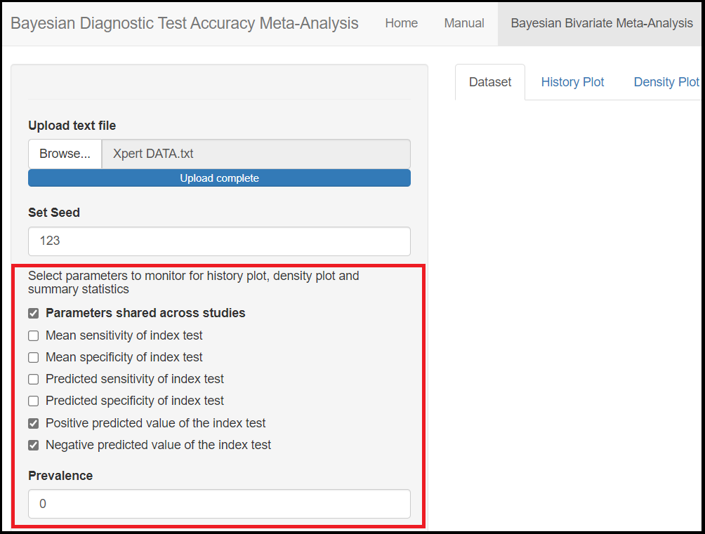
Under the Parameters shared across studies check box,
Mean sensitivity of index test(later referred asMean_Sein the results)Mean specificity of index test(later referred asMean_Spin the results)Predicted sensitivity of index test(later referred asPredicted_Sein the results)Predicted specificity of index test(later referred asPredicted_Spin the results)
Under the Parameters varying across studies check box,
Sensitivity of index test(later referred assein the results)Specificity of index test(later referred asspin the results)
Under the Shared parameters on the logit scale check box,
Mean logit (Sensitivity) of index test(later referred asmu[1]in the results)Mean logit (specificity) of index test(later referred asmu[2]in the results)Between-study precision in logit (Sensitivity) of index test(later referred asprec[1]in the results)Between-study precision in logit (specificity) of index test(later referred asprec[2]in the results)Correlation between logit sensitivity and logit specificity(later referred asrhoin the results)
Actually, the only parameters that are not being monitored by default are the Positive predicted value of the index test and Negative predicted value of the index test parameters under the Parameters shared across studies check box. In order to monitor them, the user must check the Parameters shared across studies box which will enable more check box options, including the Positive predicted value of the index test and Negative predicted value of the index test options. To tell the app you want to monitor them, you will check those boxes which will enable the option to specify a guess value for the disease Prevalence. By entering a value between 0 and 1, this will enable the app to monitor the positive and negative predicted values.
OPTIONAL SETTINGS
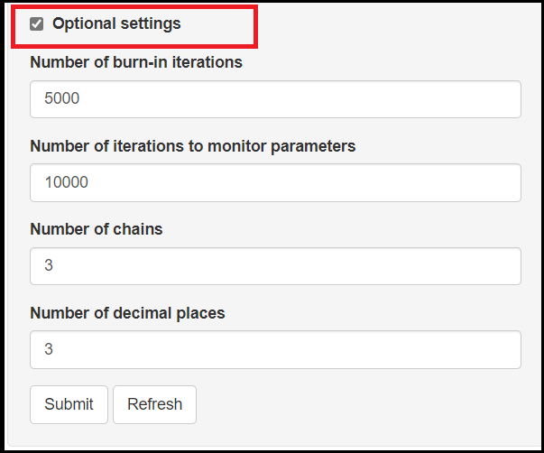
The bottom check box option, named Optional settings provides the user with more control over the MCMC process with options like
- Setting the
Number of burn-in iterations. It consists of a number of iterations that are discarded during the early MCMC sampling process. The default setting is to discard the first 5,000 iterations. - Seeting the
Number of iterations to monitor parameters. This controls how many iterations will be perform to create the posterior sample of each parameter. The default number of iterations is 10,000. - Setting the
Number of chains. In a MCMC run, the current iteration value of a given parameter, depends on the previously drawn value and so on, such that all those values form what we call a chain. Therefore, this provides the user with the option to control how many chains to monitor. Selecting to have more than 1 chain will generally help assess convergence. The default is to monitor 3 chains. - Setting the
Number of decimal places. This option allows the user to determine how precise they want the results to be. The default is to display 3 digits.
SUBMIT AND REFRESH BUTTONS
At the bottom of the page, the Submit and Refresh buttons will launch the MCMC iterative sampling process and clear the app in order to start from scratch, respectively. On the right side beneath the 4 main tab menus, there are 5 sub-tab menus. Those are the tab menus reserved for the result outputs and will only be filled once after the Submit button has been pressed.
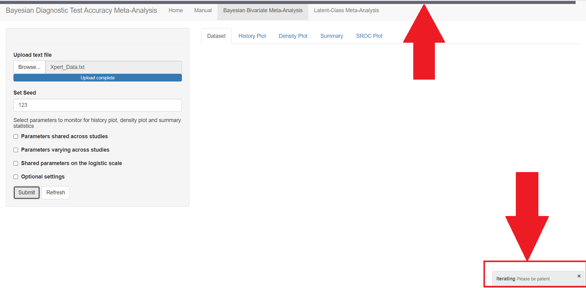
When the app is running the MCMC iterative sampling process (after having pressed the Submit button), there are 2 visible signs that the app is running in the background. First, at the top of the app, you will see a progress bar moving back and fourth, ensuring that the app isn’t stuck. The other sign appears in the lower right corner. The app will display a small window with the words Iterating Please be patient. The time the app takes to run will largely vary with the number of studies, the number of iterations to monitor parameters and the model used (Bayesian Bivariate Meta-Analysis or Latent-Class Meta-Analysis tab menu).
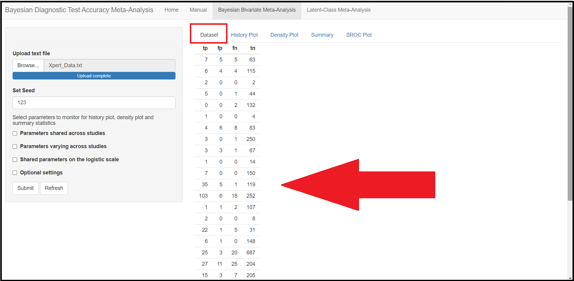
DATA TAB MENU
Once the app has finished running in the background, the Data tab menu will get filled with the complete data file that was uploaded earlier in the LOADING THE DATA sub-section.
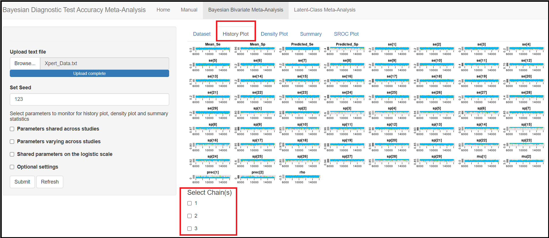
HISTORY PLOT TAB MENU
The second tab menu History Plot, will display a plot of the posterior sample values of a given parameter (Y axis) against the number of iterations (X axis). If no boxes where checked (See Monitoring Parameters subsection above), then there will be as many plots as there are parameters monitored displayed like in the figure below. Below the plots there are check box options for selecting chain(s). If no boxes are selected (the default), all chains are depicted in the parameters history plots. Although the chain selection boxes are only available in this tab menu, any boxes checked (or not) here will carry over to the other sub tab menus (Density Plot, Summary, SROC plot).
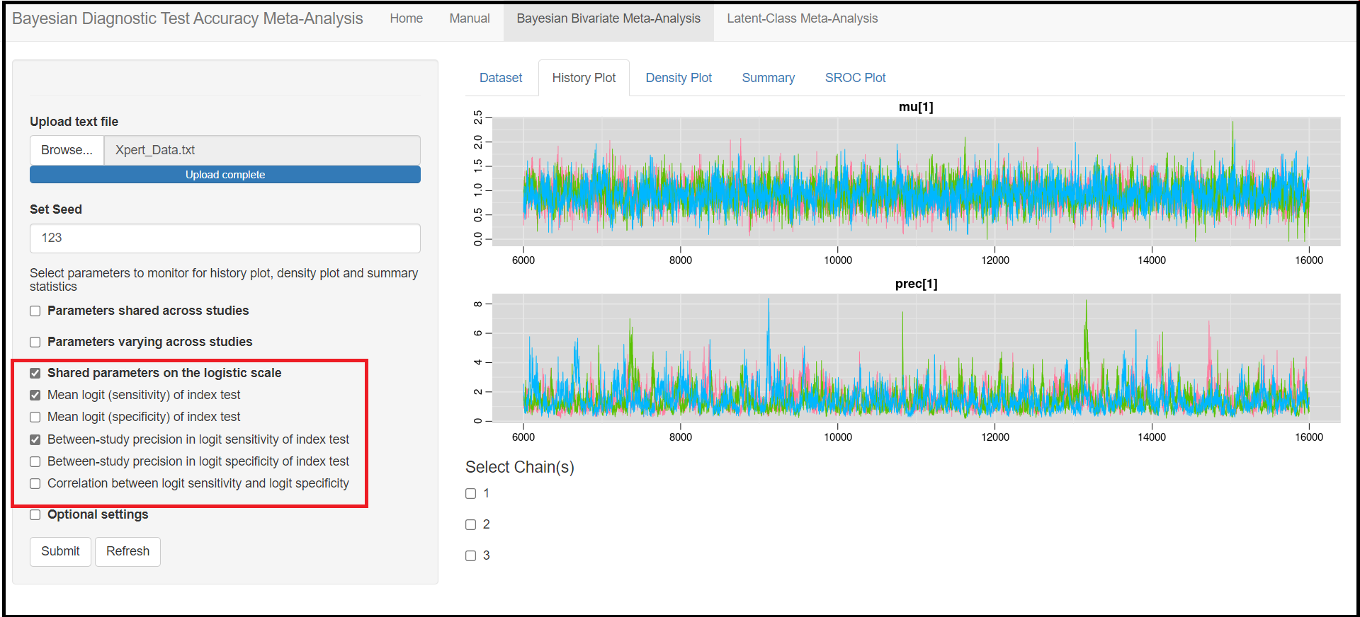
It is possible to display plots for certain parameters by selecting those specific parameters in the check box options discussed in the Monitoring Parameters sub-section. As seen in the picture below, by checking the Shared parameters on the logit scale box and then the Mean (logit) sensitivity of index test (mu[1] parameter) and Between-study precision in logit sensitivity of index test (prec[1] parameter) boxes, this will remove every other history plots from the History plot sub tab menu, except for mu[1] and prec[1].
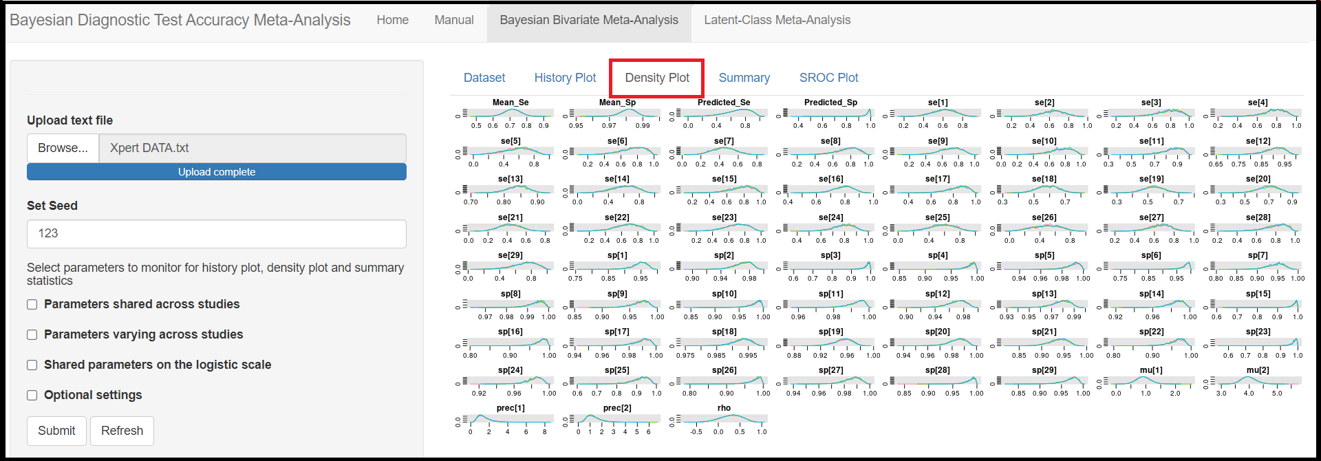
DENSITY PLOT TAB MENU
Similar to the History Plot tab menu, the Density Plot tab menu will display a plot of the posterior distribution of a given parameter based on its posterior sample. When no boxes where checked (See Monitoring Parameters subsection above), then density plots for every parameters monitored will be displayed (see figure below). When more than one chains were run, each chain will have its own density curve and they will be represented in the density plot by overlapping density curves of different colors. Recall that the check box options for selecting chain(s) can be found in the History Plot.
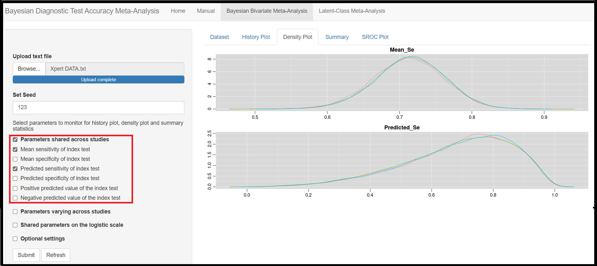
Zoom-in of certain parameter density plots can be achieved by selecting those specific parameters in the check box options discussed in the Monitoring Parameters sub-section. For instance, by checking the Parameters shared across studies box and then the Mean sensitivity of index test (Mean_Se parameter) and Predicted sensitivity of index test (Predicted_Se parameter) boxes, only the density plots for Mean_Se and Predicted_Se will be displayed in the Density plot sub tab menu (see image below).
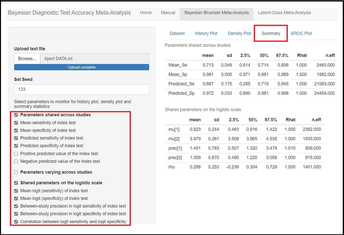
SUMMARY PLOT TAB MENU
The posterior summary statistics can be viewed in the Summary tab menu. For each parameter monitored, the following statistics are being returned:
- Mean: This is the posterior mean.
- sd: The posterior standard deviation.
- 2.5%: The 2.5% posterior quantile.
- 50%: The 50% posterior quantile, also referred to the posterior median.
- 97.5%: The 97.5% posterior quantile.
- Rhat: The Gelman-Rubin statistic. It is enabled when 2 or more chains are generated. It evaluates MCMC convergence by comparing within- and between-chain variability for each model parameter. Rhat tends to 1 as convergence is approached (Gelman and Rubin[-@Gelman1992], Brooks and Gelman[-@Brooks1998]).
- n.eff: The effective sample size. Because the MCMC process causes the posterior draws to be correlated, the effective sample size is an estimate of the sample size required to achieve the same level of precision if that sample was a simple random sample. When draws are correlated, the effective sample size will generally be lower than the actual numbers of draws resulting in poor posterior estimates (Gelman et al[-@Gelman2013]).
The 2.5% and 97.5% posterior quantiles are commonly reported as the 95% credible interval.
SROC PLOT TAB MENU
The final sub tab menu is the SROC PLOT tab menu. By default, it will plot each individual studies (blue shaded squares) as well as a summary point (black circle with coordinates (Mean_Sp, Mean_Se)) in a ROC space. The blue squares are proportional to the sample size of their respective study, with the largest squares corresponding to the largest studies.
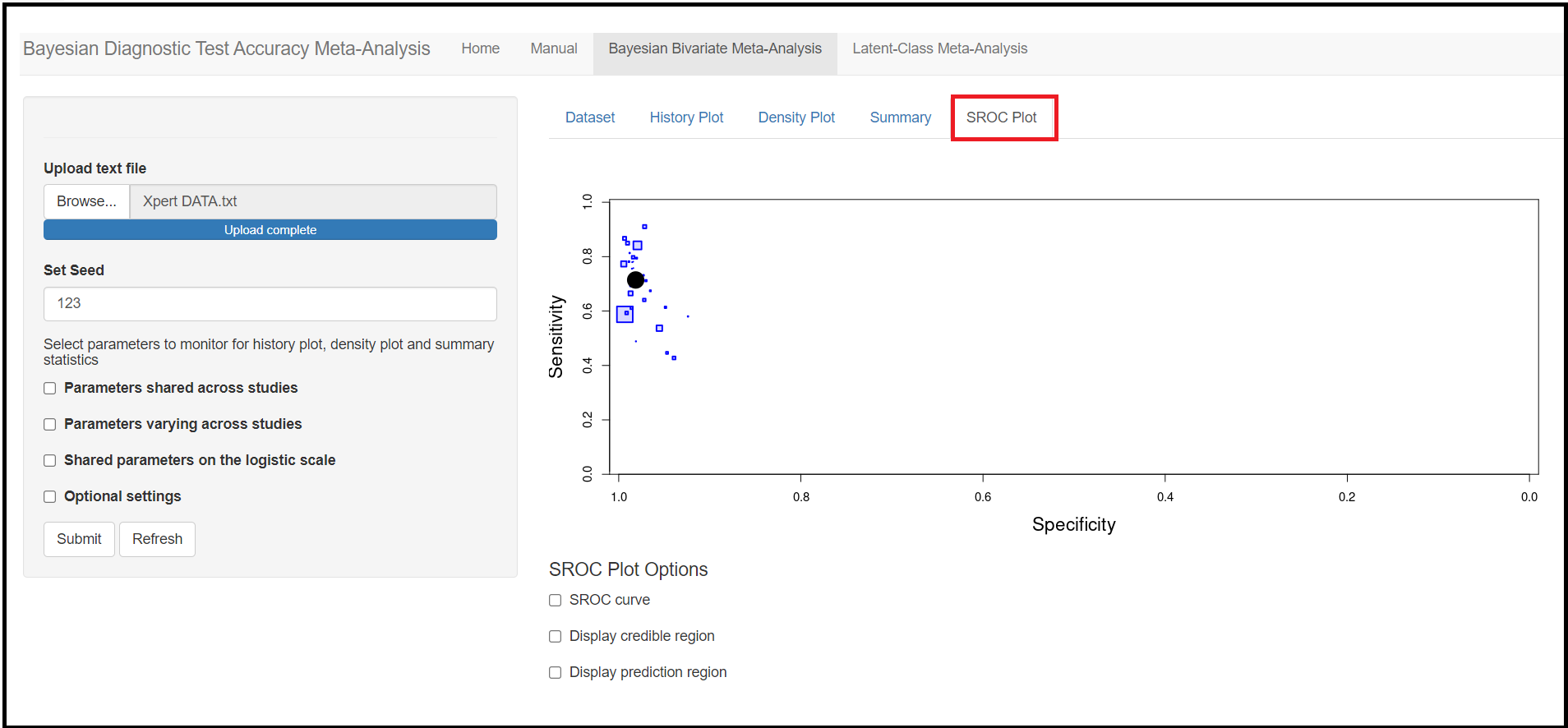
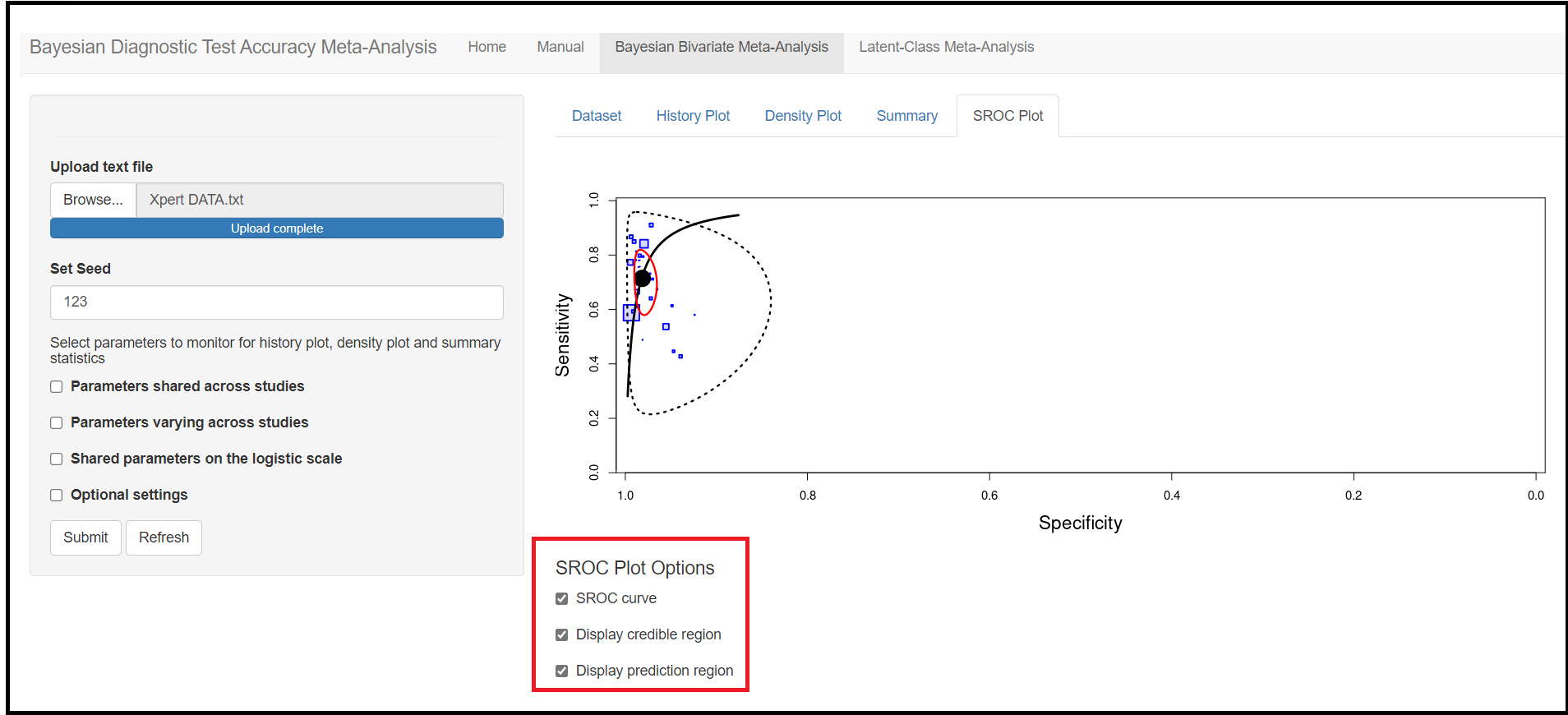
Further options below the plot allows the user to customize the figure by adding an SROC curve, credible and/or prediction regions.
In order to create the SROC curve, the conversion from bivariate parameters to HSROC parameters is done according to Harbord([-@Harbord2007]). The calculation of the credible and prediction regions are also derived from that paper.
LATENT CLASS META-ANALYSIS
Like in the Bayesian bivariate model, we are still interested in estimating the index test’s propertises, but the main difference is that we are now acknowledging that the reference test is imperfect. This model is referred to as latent class model and it extends the bivariate model by allowing the reference test to be imperfect (Xie et al[-@Xie2017], Dendukuri et al[-@Dendukuri2012]). This model is accessible under the Latent-Class Meta-Analysis tab menu.
 The
The Latent-Class Meta-Analysis tab menu shares a certain number of options with the Bayesian Bivariate Meta-Analysis tab menu. In this section, we will therefore highlights the new options that are related to the latent class model. Anything not covered here works exactly as in the Bayesian Bivariate Meta-Analysis tab menu.
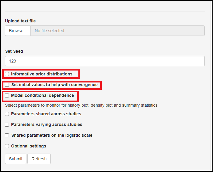
The first visual differences with the Bayesian Bivariate Meta-Analysis tab menu are the presence of new check boxes underneath the Set Seed option. The new options are as follow:
Informative prior distributioncheck box.
Set initial values to help convergencecheck box.Model conditional dependencecheck box.
We will go over those 3 new options in the next sub sections
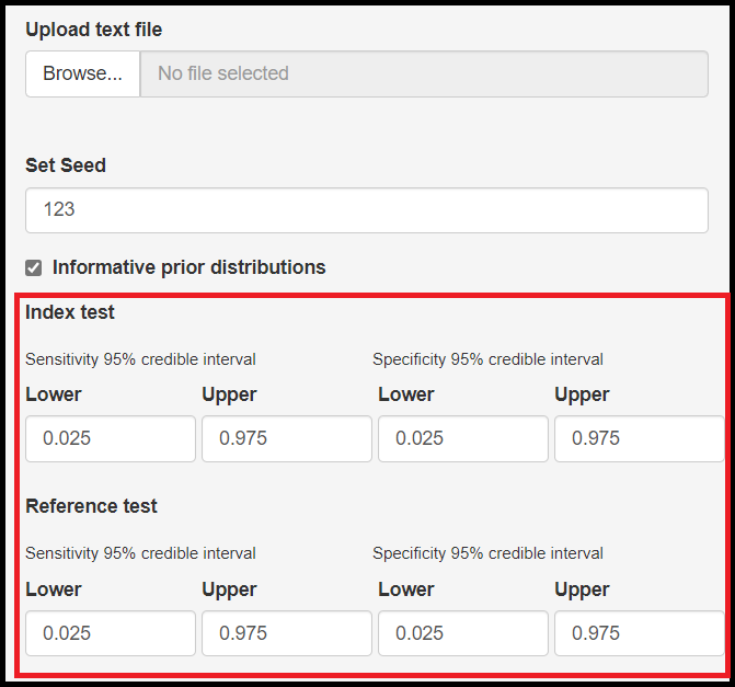
Informative prior distribution check box
Through our many years of experience working with these models, we found that the latent class models can be sensitive to prior information. The app allows certain freedom for that by giving the option to tweak prior information for the index and reference tests. So when checking the box (as seen in the image below), you will be given with specifying the lower and upper limit of a 95% credible interval for sensitivity and/or specificity. Nothing is being estimated at this step as this is based on prior knowledge one might have on the test’ sensitivity and specificity. So for instance, if it is believed that the sensitivity ranges between 0.6 and 0.8 with probability 0.95, then Lower should bet set to 0.6 and Upper sould be equal to 0.8. So bascially, if any prior knowledge exists, it can pay off to include it in the model at this step. Otherwise, the default values Lower=0.025 and Upper=0.975 were selected such that the prior is approximately uniform over the range [0,1], which corresponds to a vague prior. This vague prior is also used by default if the Informative prior distribution box is left unchecked.
For the more advanced user who wants to connect this with the theory behind the model, this uniform prior on sensitivity/specificity corresponds to a normal prior with mean=0 and variance=4 placed on the logit-transformed sensitivity/specificity.
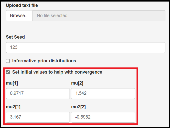
Set initial values to help with convergence check box
Latent class models can also be affected by the starting values. To mitigate that, the app allows to setup initial values for the following parameters:
- Mean logit sensitivity of the index test, noted by
mu[1] - Mean logit specificity of the index test, noted by
mu[2] - Mean logit sensitivity of the reference test, noted by
mu2[1] - Mean logit specificity of the reference test, noted by
mu2[2]
There are no “one size fit all” set of initial values here. The app provides some by default, but the user should really not rely on them and instead provide the ones that makes more sense from their own model perspective.
Contrary to the prior check box in the previous sub-section, here the initial values must be supplied on the logit scale which might not be intuitive at first. As a guide line, keep in mind that a value of 0 on the logit scale back-transforms into 0.50 on the probability scale. This means that if you want to select an initial value of 0.50 for the sensitivity of the reference test, then you would have to enter the value 0 under the mu2[1] box. Keeping that logic in mind, if we increase values on the logit scale above 0 we get closer to a probability of 1. Similarly, decreasing the logit scale value below 0 (negative values), we get closer to a probability of 0.
Here are some more examples:
- A value of 0 on the logit scale corresponds to a probability of 0.5
- A value of 1 on the logit scale corresponds to a probability of 0.7310586
- A value of 1.25 on the logit scale corresponds to a probability of 0.7772999
- A value of 2 on the logit scale corresponds to a probability of 0.8807971
- A value of 3 on the logit scale corresponds to a probability of 0.9525741
- A value of -1 on the logit scale corresponds to a probability of 0.2689414
- A value of -1.25 on the logit scale corresponds to a probability of 0.2227001
- A value of -2 on the logit scale corresponds to a probability of 0.1192029
- A value of -3 on the logit scale corresponds to a probability of 0.0474259
For the more advanced user, the equation transforming a probability onto a logit value is given by the following expression
\[ l = log\left( \frac{p}{1-p} \right), \] where \(l\) and \(p\) are the logit and probability values respectively.
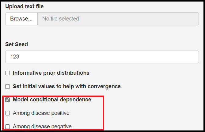
Model conditional dependence check box
When the reference test is no longer assumed to be perfect, it means that it is likely to make some errors, i.e. being positive when the subject receiving the test is actually free of the disease (commonly referred to as a false positive result) or come out negative when the subject does have the disease (a false negative result). When both the reference test and the index test are making the same error, this is referred to as conditional dependence.
It is possible to allow for conditional dependence by checking the Model conditional dependence check box. By doing so, it will prompt 2 new check boxes which basically allow the user to select what type of error both the index and reference tests are believed to make more often simultaneaously.
Among disease positivecheck box means that the conditional dependence is occurring due to false negative resultsAmong disease negativecheck box means that the conditional dependence is occurring due to false positive results
Extra parameters of the model
Modelling the reference test to be imperfect means that our latent class model has more parameters than the simpler Bayesian bivariate model. In this section we simply highlight the new parameters that are monitored by the model with their labels for easy reference in the Summary tab menu.
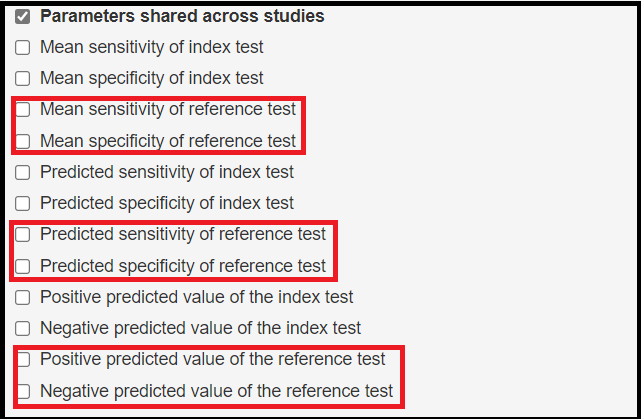
The following parameters shared across studies are being added by the latent class model.
- Mean sensitivity of reference test denoted by
mu2[1] - Mean specificity of reference test denoted by
mu2[2] - Predicted sensitivity of reference test denoted by
Predicted_Se2 - Predicted specificity of reference test denoted by
Predicted_Sp2 - Positive predicted value of the reference test denoted by
Summary_PPV2 - Negative predicted value of the reference test denoted by
Summary_NPV2
As we have seen in the Monitoring parameters subsection of the Bayesian bivariate model section above, Summary_PPV2 and Summary_NPV2 will not be monitored by default unless their respective boxes were checked before running the app.
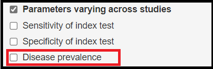
The model also monitors disease prevalence parameters for every study. This means that the parameters varying across studies will add a bunch of disease prevalence parameters that will be denoted by prev indexed by the study number, i.e. prev[1] for the estimate of the disease prevalence of the first study, prev[2] for the estimate of the disease prevalence of the second study and so on.
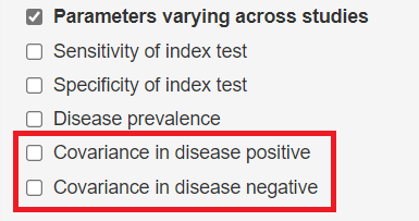
If conditional dependence was modeled as seen in the Model conditional dependence subsection, then 2 extra check boxes will become available under the Parameters varying across studies check box option. By default, the summary statistics for both covariance terms will not appear in the various output tabs unless the 2 boxed are properly checked. Similar to the disease prevalence, there will be as many covariance terms as there are studies.
- Covariance in disease positive will be denoted by
covpindexed by the study number, i.e.covp[1]for the covariance in disease positive for study 1,covp[2]for the covariance in disease positive for study 2, so on.
- Covariance in disease negative will be denoted by
covnindexed by the study number, i.e.covn[1]for the covariance in disease negative for study 1,covn[2]for the covariance in disease negative for study 2, so on.
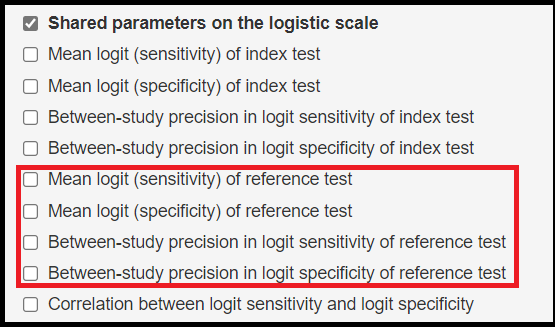
Finally, the following shared parameters on the logit scale will also be added by default to the list of parameters monitored as part of the latent class model:
- Mean logit (Sensitivity) of reference test denoted by
mu2[1] - Mean logit (specificity) of reference test denoted by
mu2[2] - Between-study precision in logit sensitivity of reference test denoted by
prec2[1] - Between-study precision in logit specificity of reference test denoted by
prec2[2]
REFERENCES
Citation
@online{schiller2021,
  author = {Ian Schiller and Nandini Dendukuri},
  title = {How-to Guide on {R} {Shiny} App for {Bayesian} {Diagnostic}
    {Test} {Meta-Analysis}},
  date = {2021-11-17},
  url = {https://www.nandinidendukuri.com/blogposts/2021-11-17-bayesdta-shiny-app/},
  langid = {en}
}