OVERVIEW
Through this blog, we will look at each step of a program in the R language (R Core Team Team (2020)). The program uses the rjags package (an interface to the JAGS library (Plummer Plummer (2003) ) in order to draw samples from the posterior distribution of the parameters using Markov Chain Monte Carlo (MCMC) methods. The program relies on the mcmcplots package to assess convergence of the meta-analysis model. The meta-analtsis model returns the parameters of the SROC curve across studies. The SROC curve can be created using the DTAplots package.
MOTIVATING EXAMPLE AND DATA
This script will illustrate the method by application to data from a systematic review of 37 studies evaluating the accuracy of Anti-cyclic citrullinated peptide (Anti-CCP) test for rheumatoid arthritis (index test) compared to the 1987 revised American college of Rheumatology (ACR) criteria for clinical diagnosis (reference test) (Nishimura et al Nishimura et al. (2007)). Each study provided a two-by-two table of the form
| Disease_positive | Disease_negative | |
|---|---|---|
| Inex test positive | TP | FP |
| Index test negative | FN | TN |
where:
TPis the number of individuals who tested positive on both testsFPis the number of individuals who tested positive on the index test and negative on the reference testFNis the number of individuals who tested negative on the index test and positive on the reference testTNis the number of individuals who tested negative on both tests
TP=c(64, 482, 36, 143, 80, 61, 27, 60, 261, 20, 42, 18, 8, 93, 143,
     84, 30, 32, 70, 48, 75, 64, 32, 130, 50, 20, 77, 73, 36, 56,
     115, 49, 22, 8, 35, 161, 80, 5, 57, 383, 89, 57, 196, 163, 75,
     157, 26, 62, 113, 25)
FP=c(16, 2, 6, 43, 50, 36, 6, 8, 54, 2, 46, 3, 8, 28, 39, 41, 2,
     29, 39, 1, 42, 18, 10, 8, 14, 32, 16, 22, 3, 11, 53, 23, 2, 8,
     8, 89, 28, 4, 9, 38, 3, 25, 75, 10, 21, 287, 1, 11, 19, 1)
FN=c(27, 82, 41, 53, 39, 37, 3, 20, 63, 29, 14, 31, 0, 25, 63, 56,
     23, 3, 36, 40, 12, 29, 9, 128, 20, 26, 52, 29, 5, 46, 67, 28,
     20, 31, 51, 7, 69, 11, 33, 166, 9, 6, 99, 28, 21, 78, 32, 114,
     29, 14)
TN=c(153, 153, 313, 196, 45, 196, 33, 119, 197, 18, 127, 25, 31,
     118, 130, 90, 73, 13, 93, 99, 191, 73, 13, 113, 191, 25, 52,
     90, 70, 87, 63, 359, 80, 91, 149, 360, 284, 49, 93, 170, 39,
     111, 345, 140, 106, 1466, 29, 127, 481, 20)

pos= TP + FN
neg= TN + FP

n <- length(TP) #  Number of studies

dataList = list(TP=TP,TN=TN,n=n,pos=pos,neg=neg)
THE MODEL
Before moving any further, let’s look briefly at the theory behind the hierarchical meta-analysis model. An HSROC model assumes that there is an underlying ROC curve in each study behind the observed data.
Within-study level: In each study, the TP and TN entries of the 2x2 table are assumed to follow a binomial distribution with probabilities (on logit scale) respectively expressed as follows :
\[ logit(se_i) = \left(\theta_i + \frac{\alpha_i}{2} \right)e^{-\frac{\beta}{2}} \]
\[ logit(sp_i) = \left(-\theta_i + \frac{\alpha_i}{2} \right)e^{\frac{\beta}{2}}\]
where \(se_i\) and \(sp_i\) are the sensitivity and specificity in study \(i\) respectively, \(\theta_i\) represents the positivity threshold in study \(i\), \(\alpha_i\) represents a measure of diagnsotic accuracy in the \(i^{th}\) study and \(\beta\) (the shape parameter) provides for asymmetry in the ROC curve by allowing accuracy to vary with threshold. It is assumed that \(\beta\) is the same in each study.
Between-study level: For each study, both \(\theta_i\) and \(\alpha_i\) are assumed to follow a normal distribution:
\[ \theta_i \sim N(\Theta, \tau_{\theta})\]
\[ \alpha_i \sim N(\Lambda, \tau^2_{\alpha})\]
where \(\Theta\) is the average positivity threshold, \(\Lambda\) is the mean accuracy, \(\tau_{\theta}\) and \(\tau^2_{\alpha}\) are the precision parameters for the positivity threshold and accuracy respectively. Variances for both positivity threshold and accuracy parameter can be derived from the precision parameters as \(\sigma^2_{\theta} = \frac{1}{\tau_{\theta}}\) and \(\sigma^2_{\alpha} = \frac{1}{\tau_{\alpha}}\), respectively.
To carry out Bayesian estimation, we need to specifyprior distributions over the unknown parameters, namely, for \(\Theta\), \(\Lambda\), \(\beta\), \(\tau_{\theta}\) and \(\tau_{\alpha}\). Prior distributions for those parameters are usually selected to be vague with the intention that they have a negligible impact on the results.
The model is written in JAGS syntax, and stored in a character object that we called modelString which is later saved in the current working directory via the R function writeLines as follow.
# HSROC model
modelString =
"
model {
# === LIKELIHOOD === #
for(i in 1:n) {
TP[i] ~ dbin(se[i],pos[i])
TN[i] ~ dbin(sp[i],neg[i])
# === HIERARCHICAL PRIOR === #
logit(se[i]) <- (theta[i] + 0.5*alpha[i])/exp(beta/2)
logit(sp[i]) <- (-theta[i] + 0.5*alpha[i])*exp(beta/2)
theta[i] ~ dnorm(THETA,prec[2])
alpha[i] ~ dnorm(LAMBDA,prec[1])
}
### === HYPER PRIOR DISTRIBUTIONS === ###
THETA ~ dunif(-10,10)
LAMBDA ~ dunif(-2,20)
beta ~ dunif(-5,5)
for(i in 1:2) {
prec[i] ~ dgamma(2.1,2)
tau.sq[i] <- 1/prec[i]
tau[i] <- pow(tau.sq[i],0.5)
}
}
"

writeLines(modelString,con="model.txt")
INTIAL VALUES
To assess convergence of the MCMC algorithm, we recommend running multiple chains, each starting at different initial values in order to examine if all chains reach the same solution. There are different ways of providing initial values. In the illustration below we give details on how to provide initial values chosen by the user by using a function we created and called GenInits().
Providing relevant initial values can speed up convergence of the MCMC algorithm. The function we created allows us to provide our own initial values for the average positivity threshold (THETA), the mean accuracy (LAMBDA) as well as the shape parameter (beta). We can provide specific initial values to THETA, LAMBDA and beta through the THETA, LAMBDA and beta arguments respectively or we can use the function to randomly generate initial values from distributions corresponding to the prior distribution found in the model for THETA, LAMBDA and beta. In this example, we have allowed other parameters, such as precision parameters (prec[1] and prec[2]) to be randomly generated by GenInits(). In our experience, choosing initial values for these parameters is not easy. For reproducibility, a Seed argument is provided.
In the illustration below, for all chains we simply set the arguments THETA, LAMBDA and beta to NULL. This ensure the chains are randomly initialized.
# Initial values
GenInits = function(Seed=seed, THETA=NULL, LAMBDA=NULL, beta=NULL){
        if(is.null(THETA) == "FALSE" & is.null(LAMBDA) == "FALSE" & is.null(beta) == "FALSE"){
                THETA=THETA;
                LAMBDA=LAMBDA;
                beta=beta;
        }
        else{
                THETA = runif(1, -10, 10);
                LAMBDA = runif(1, -2, 20);
                beta = runif(1, -5, 5) ;
        }
        list(
                THETA = THETA,
                LAMBDA = LAMBDA,
                beta = beta,
                prec = rep(rgamma(1,shape=2.1,rate=2), 2),
                .RNG.name="base::Wichmann-Hill",
                .RNG.seed=Seed
        )
}
seed=8; set.seed(seed)
Listinits = list(
        GenInits(),
        GenInits(),
        GenInits(),
        GenInits(),
        GenInits()
)
COMPILING AND RUNNING THE MODEL
The jags.model function compiles the model to check for possible syntax error. Argument n.chains=5 creates 5 MCMC chains with different starting values given by the Listinits object defined above. At this step, jags.model is said to be in adaptive mode in order to ensure optimal sampling behaviour in the later steps. By default, it will run and discard 1,000 iterations. This value can be tweaked with the n.adapt argument. (See Section 3.4 of the JAGS manual for further details.)
library(rjags)
# Compile the model
jagsModel = jags.model("model.txt",data=dataList,n.chains=5,inits=Listinits)
The update function serves as to carry out the “burn-in” step. This corresponds to discarding initial iterations till the MCMC algorithm has reached its equilibrium distribution. Here we chose to discard 30,000 iterations by providing argument n.iter=30000. This can be helpful to mitigate “bad” initial values.
# Burn-in iterations
update(jagsModel,n.iter=30000)
The coda.samples function draws samples from the posterior distribution of the unknown parameters that were defined in the parameters object. Here we are drawing n.iter=30000 iterations from the posterior distributions for each chain.
# Parameters to be monitored
parameters = c("se", "sp", "alpha", "theta", "prec", "tau.sq", "tau", "THETA", "LAMBDA", "beta")
# Posterior samples
output = coda.samples(jagsModel,variable.names=parameters,n.iter=30000)
MONITORING CONVERGENCE
Convergence of the MCMC algorithm can now be examined. The code below will create a 3-panel plot consisting of the density plot, the running mean plot and a history plot for parameters that vary across studies, e.g. \(\theta_i\) and \(\alpha_i\) in each study.
library(mcmcplots)
# Plots to check convergence for parameters varying across studies:
# Index j refers to the number of studies
# Index i follows the ordering of the parameters vector defined above.  If left unchanged :
# i = 1 : logit-transformed sensitivity in study j (se)
# i = 2 : logit-transformed specificity in study j (sp)
# i = 3 : accuracy in study j (alpha)
# i = 4 : positivity threshold in study j (theta)

for(j in 1:n) {
        for(i in 1:4) {
                par(oma=c(0,0,3,0), mar=c(2,2,2,2))
                layout(matrix(c(1,2,3,3), 2, 2, byrow = TRUE))
                denplot(output, parms=c(paste(parameters[i],"[",j,"]",sep="")), auto.layout=FALSE, main="(a)", xlab=paste(parameters[i],"",sep=""), ylab="Density")
                rmeanplot(output, parms=c(paste(parameters[i],"[",j,"]",sep="")), auto.layout=FALSE, main="(b)")
                title(xlab="Iteration", ylab="Running mean")
                traplot(output, parms=c(paste(parameters[i],"[",j,"]",sep="")), auto.layout=FALSE, main="(c)")
                title(xlab="Iteration", ylab=paste(parameters[i],"[",j,"]",sep=""))
                mtext(paste("Diagnostics for ", parameters[i],"[",j,"]","",sep=""), side=3, line=1, outer=TRUE, cex=2)

        }
}
Then we create the same 3-panel plot for the parameters that are shared across studies.
# Plots to check convergence for parameters shared across studies:
# Index j = 1 refers to accuracy parameter and j = 2 refers to cut-off value for defining a positive test
# Index i follows the ordering of the parameters vector defined above. If left unchanged :
# i = 5 : precision of the accuracy parameter (j=1) and precision of the positivity threshold parameter (j=2) (prec)
# i = 6 : variance of the accuracy parameter (j=1) and variance of the positivity threshold parameter (j=2) (tau.sq)
# i = 7 : standard deviation of the accuracy parameter (j=1) and standard deviation of the positivity threshold parameter (j=2) (tau)
for(j in 1:2) {
for(i in 5:7) {
par(oma=c(0,0,3,0))
layout(matrix(c(1,2,3,3), 2, 2, byrow = TRUE))
denplot(output, parms=c(paste(parameters[i],"[",j,"]",sep="")), auto.layout=FALSE, main="(a)", xlab=paste(parameters[i],"",sep=""), ylab="Density")
rmeanplot(output, parms=c(paste(parameters[i],"[",j,"]",sep="")), auto.layout=FALSE, main="(b)")
title(xlab="Iteration", ylab="Running mean")
traplot(output, parms=c(paste(parameters[i],"[",j,"]",sep="")), auto.layout=FALSE, main="(c)")
title(xlab="Iteration", ylab=paste(parameters[i],"[",j,"]",sep=""))
mtext(paste("Diagnostics for ", parameters[i],"[",j,"]","",sep=""), side=3, line=1, outer=TRUE, cex=2)
}
}
# Index j not needed for the following shared parameters
# i = 8 : mean positivity threshold parameter (THETA)
# i = 9 : mean accuracy parameter (LAMBDA)
# i = 10: shape parameter (beta)
for(i in 8:10) {
par(oma=c(0,0,3,0))
layout(matrix(c(1,2,3,3), 2, 2, byrow = TRUE))
denplot(output, parms=c(paste(parameters[i], sep="")), auto.layout=FALSE, main="(a)", xlab=paste(parameters[i],"",sep=""), ylab="Density")
rmeanplot(output, parms=c(paste(parameters[i], sep="")), auto.layout=FALSE, main="(b)")
title(xlab="Iteration", ylab="Running mean")
traplot(output, parms=c(paste(parameters[i], sep="")), auto.layout=FALSE, main="(c)")
title(xlab="Iteration", ylab=paste(parameters[i], sep=""))
mtext(paste("Diagnostics for ", parameters[i], sep=""), side=3, line=1, outer=TRUE, cex=2)
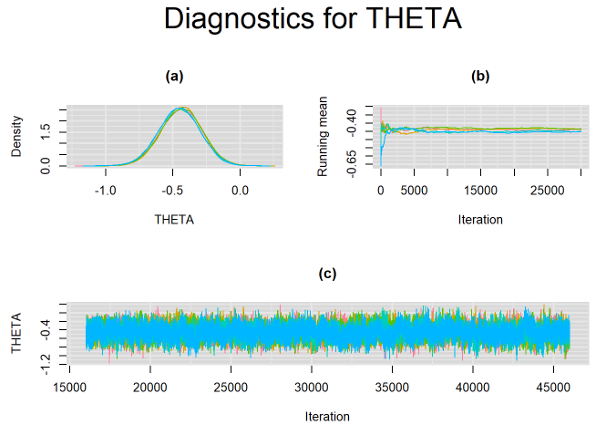
}For example, in the figure below, the posterior densities (a), running posterior mean values (b) and history plots (c) for the parameter THETA (mean positivity threshold) is displayed for each chain represented by different color. The very similar results from all five chains suggest the algorithm has converged to the same solution in each case.
SUMMARY STATISTICS
Once convergence of the MCMC algorithm is achieved, summary statistics of the parameters of interest may be extracted from their posterior distributions using the MCMCsummary function found in the MCMCvis package.
# Summary statistics
# Summary statistics
MCMCsummary(output, params=c("THETA", "LAMBDA", "beta","tau.sq", "prec"), round=4)
Below is the summary statistics output for the parameters shared across studies. The 50% quantile is the posterior median which is commonly used to estimate the paramater of interest. Its corresponding 95% credible interval is given by the 2.5% and 97.5% quantiles.
The table also displays Rhat, which is the Gelman-Rubin statistic (Gelman and Ruben Gelman and Rubin (1992), Brooks and Gelman Brooks and Gelman (1998) ). It is enabled when 2 or more chains are generated. It evaluates MCMC convergence by comparing within- and between-chain variability for each model parameter. Rhat tends to 1 as convergence is approached.
Also, n.eff is the effective sample size (Gelman et al Gelman et al. (2013) ). Because the MCMC process causes the posterior draws to be correlated, the effective sample size is an estimate of the sample size required to achieve the same level of precision if that sample was a simple random sample. When draws are correlated, the effective sample size will generally be lower than the actual numbers of draws resulting in poor posterior estimates
# Summary statistics
library(MCMCvis)
library(DT)
datatable(MCMCsummary(output, round=4), options = list(pageLength = 3) )
SROC PLOT
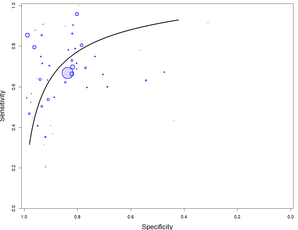
The output from rjags can be used to create a summary receiver operating characteristic (SROC) curve (black line) using the SROC_rjags function found in the DTAplots package. Sensitivity and specificity estimates from individual studies are represented by circles with diameter proportional to the study sample size.
# SROC plot
library(DTAplots)
SROC_rjags(X=output, model="HSROC",n=n, study_col1="blue", study_col2=rgb(0, 0, 1, 0.15), dataset=cbind(TP,FP,FN,TN), ref_std=TRUE, Sp.range=c(0,1), SROC_curve = TRUE, cred_region = FALSE, predict_region = FALSE)
SCRIPT
Below is a copy of the complete script to run the Bayesian HSROC meta-analysis model in rjags.
####################################
#### DATA FOR MOTIVATING EXAMPLE ###
####################################
TP=c(64, 482, 36, 143, 80, 61, 27, 60, 261, 20, 42, 18, 8, 93, 143,
     84, 30, 32, 70, 48, 75, 64, 32, 130, 50, 20, 77, 73, 36, 56,
     115, 49, 22, 8, 35, 161, 80, 5, 57, 383, 89, 57, 196, 163, 75,
     157, 26, 62, 113, 25)
FP=c(16, 2, 6, 43, 50, 36, 6, 8, 54, 2, 46, 3, 8, 28, 39, 41, 2,
     29, 39, 1, 42, 18, 10, 8, 14, 32, 16, 22, 3, 11, 53, 23, 2, 8,
     8, 89, 28, 4, 9, 38, 3, 25, 75, 10, 21, 287, 1, 11, 19, 1)
FN=c(27, 82, 41, 53, 39, 37, 3, 20, 63, 29, 14, 31, 0, 25, 63, 56,
     23, 3, 36, 40, 12, 29, 9, 128, 20, 26, 52, 29, 5, 46, 67, 28,
     20, 31, 51, 7, 69, 11, 33, 166, 9, 6, 99, 28, 21, 78, 32, 114,
     29, 14)
TN=c(153, 153, 313, 196, 45, 196, 33, 119, 197, 18, 127, 25, 31,
     118, 130, 90, 73, 13, 93, 99, 191, 73, 13, 113, 191, 25, 52,
     90, 70, 87, 63, 359, 80, 91, 149, 360, 284, 49, 93, 170, 39,
     111, 345, 140, 106, 1466, 29, 127, 481, 20)

pos= TP + FN
neg= TN + FP

n <- length(TP) #  Number of studies

dataList = list(TP=TP,TN=TN,n=n,pos=pos,neg=neg)

#################
### THE MODEL ###
#################
modelString =
"
model {
# === LIKELIHOOD === #
for(i in 1:n) {
TP[i] ~ dbin(se[i],pos[i])
TN[i] ~ dbin(sp[i],neg[i])
# === HIERARCHICAL PRIOR === #
logit(se[i]) <- (theta[i] + 0.5*alpha[i])/exp(beta/2)
logit(sp[i]) <- (-theta[i] + 0.5*alpha[i])*exp(beta/2)
theta[i] ~ dnorm(THETA,prec[2])
alpha[i] ~ dnorm(LAMBDA,prec[1])
}
### === HYPER PRIOR DISTRIBUTIONS === ###
THETA ~ dunif(-10,10)
LAMBDA ~ dunif(-2,20)
beta ~ dunif(-5,5)
for(i in 1:2) {
prec[i] ~ dgamma(2.1,2)
tau.sq[i] <- 1/prec[i]
tau[i] <- pow(tau.sq[i],0.5)
}
}
"

writeLines(modelString,con="model.txt")

######################
### INITIAL VALUES ###
######################
GenInits = function(Seed=seed, THETA=NULL, LAMBDA=NULL, beta=NULL){
        if(is.null(THETA) == "FALSE" & is.null(LAMBDA) == "FALSE" & is.null(beta) == "FALSE"){
                THETA=THETA;
                LAMBDA=LAMBDA;
                beta=beta;
        }
        else{
                THETA = runif(1, -10, 10);
                LAMBDA = runif(1, -2, 20);
                beta = runif(1, -5, 5) ;
        }
        list(
                THETA = THETA,
                LAMBDA = LAMBDA,
                beta = beta,
                prec = rep(rgamma(1,shape=2.1,rate=2), 2),
                .RNG.name="base::Wichmann-Hill",
                .RNG.seed=Seed
        )
}
seed=8; set.seed(seed)
Listinits = list(
        GenInits(),
        GenInits(),
        GenInits(),
        GenInits(),
        GenInits()
)


#######################################
### COMPILING AND RUNNING THE MODEL ###
#######################################
jagsModel = jags.model("model.txt",data=dataList,n.chains=5,inits=Listinits)
# Burn-in iterations
update(jagsModel,n.iter=30000)
# Parameters to be monitored
parameters = c("se", "sp", "alpha", "theta", "prec", "tau.sq", "tau", "THETA", "LAMBDA", "beta")
# Posterior samples
output = coda.samples(jagsModel,variable.names=parameters,n.iter=30000)

##############################
### MONITORING CONVERGENCE ###
##############################
library(mcmcplots)
# Plots to check convergence for parameters varying across studies:
# Index j refers to the number of studies
# Index i follows the ordering of the parameters vector defined above.  If left unchanged :
# i = 1 : logit-transformed sensitivity in study j (se)
# i = 2 : logit-transformed specificity in study j (sp)
# i = 3 : accuracy in study j (alpha)
# i = 4 : positivity threshold in study j (theta)

for(j in 1:n) {
        for(i in 1:4) {
                par(oma=c(0,0,3,0), mar=c(2,2,2,2))
                layout(matrix(c(1,2,3,3), 2, 2, byrow = TRUE))
                denplot(output, parms=c(paste(parameters[i],"[",j,"]",sep="")), auto.layout=FALSE, main="(a)", xlab=paste(parameters[i],"",sep=""), ylab="Density")
                rmeanplot(output, parms=c(paste(parameters[i],"[",j,"]",sep="")), auto.layout=FALSE, main="(b)")
                title(xlab="Iteration", ylab="Running mean")
                traplot(output, parms=c(paste(parameters[i],"[",j,"]",sep="")), auto.layout=FALSE, main="(c)")
                title(xlab="Iteration", ylab=paste(parameters[i],"[",j,"]",sep=""))
                mtext(paste("Diagnostics for ", parameters[i],"[",j,"]","",sep=""), side=3, line=1, outer=TRUE, cex=2)

        }
}
# Plots to check convergence for parameters shared across studies:
# Index j = 1 refers to accuracy parameter and j = 2 refers to cut-off value for defining a positive test
# Index i follows the ordering of the parameters vector defined above.  If left unchanged :
# i = 5 : precision of the accuracy parameter (j=1) and precision of the positivity threshold parameter (j=2) (prec)
# i = 6 : variance of the accuracy parameter (j=1) and variance of the positivity threshold parameter (j=2) (tau.sq)
# i = 7 : standard deviation of the accuracy parameter (j=1) and standard deviation of the positivity threshold parameter (j=2) (tau)
for(j in 1:2) {
        for(i in 5:7) {
                par(oma=c(0,0,3,0))
                layout(matrix(c(1,2,3,3), 2, 2, byrow = TRUE))
                denplot(output, parms=c(paste(parameters[i],"[",j,"]",sep="")), auto.layout=FALSE, main="(a)", xlab=paste(parameters[i],"",sep=""), ylab="Density")
                rmeanplot(output, parms=c(paste(parameters[i],"[",j,"]",sep="")), auto.layout=FALSE, main="(b)")
                title(xlab="Iteration", ylab="Running mean")
                traplot(output, parms=c(paste(parameters[i],"[",j,"]",sep="")), auto.layout=FALSE, main="(c)")
                title(xlab="Iteration", ylab=paste(parameters[i],"[",j,"]",sep=""))
                mtext(paste("Diagnostics for ", parameters[i],"[",j,"]","",sep=""), side=3, line=1, outer=TRUE, cex=2)
        }
}

# Index j not needed for the following shared parameters
# i = 8 : mean positivity threshold parameter (THETA)
# i = 9 : mean accuracy parameter (LAMBDA)
# i = 10: shape parameter (beta)
for(i in 8:10) {
        par(oma=c(0,0,3,0))
        layout(matrix(c(1,2,3,3), 2, 2, byrow = TRUE))
        denplot(output, parms=c(paste(parameters[i], sep="")), auto.layout=FALSE, main="(a)", xlab=paste(parameters[i],"",sep=""), ylab="Density")
        rmeanplot(output, parms=c(paste(parameters[i], sep="")), auto.layout=FALSE, main="(b)")
        title(xlab="Iteration", ylab="Running mean")
        traplot(output, parms=c(paste(parameters[i], sep="")), auto.layout=FALSE, main="(c)")
        title(xlab="Iteration", ylab=paste(parameters[i], sep=""))
        mtext(paste("Diagnostics for ", parameters[i], sep=""), side=3, line=1, outer=TRUE, cex=2)
}

##########################
### SUMMARY STATISTICS ###
##########################
library(MCMCvis)
library(DT)
datatable(MCMCsummary(output, round=4), options = list(pageLength = 3) )

#################
### SROC PLOT ###
#################
library(DTAplots)
SROC_rjags(X=output, model="HSROC",n=n, study_col1="blue", study_col2=rgb(0, 0, 1, 0.15), dataset=cbind(TP,FP,FN,TN), ref_std=TRUE, Sp.range=c(0,1), SROC_curve = TRUE, cred_region = FALSE, predict_region = FALSE)
REFERENCES
Citation
@online{schiller2021,
  author = {Ian Schiller and Nandini Dendukuri},
  title = {Bayesian Inference for the {HSROC} Model for Diagnostic
    Meta-Analysis},
  date = {2021-05-04},
  url = {https://www.nandinidendukuri.com/blogposts/2021-05-04-HSROC-meta-analysis/},
  langid = {en}
}