| Arms | Seroconverted | Did Not Convert | Proportions of Seroconverted | 95% Confidence Interval for Each Proportion |
|---|---|---|---|---|
| High Dose | 31 | 107 | 0.225 | (0.16, 0.305) |
| Low Dose | 12 | 124 | 0.0882 | (0.046, 0.149) |
Introduction
- Sample size calculations are necessary when planning research studies.
- Typically, a guess value must be provided for the unknown parameter(s) of interest.
- Bayesian sample size calculations use prior distributions to represent uncertainty in our knowledge about the unknown parameter(s).
- The objective of this Web Demo is to illustrate Bayesian sample size calculations for estimating differences in proportions.
- We will use the R package SampleSizeProportions.
- The methods are based on the article by Joseph, Berger, and Belisle (1997).
Outline
- Assume random samples of a dichotomous variable will be collected from each of two independent populations with the goal of estimating the difference in the “probability of success” between them.
- The prior distribution is used to generate a large number of possible datasets we may observe for a given sample size.
- For each dataset we calculate the posterior credible interval of the difference between the proportions.
- We examine the coverage and/or length of the credible interval across the datasets to see if they have the precision and coverage we desire.
- By comparing results for different sample sizes, we find the desired sample size.
Motivating Example
- We wish to design a study to estimate the efficacy of a flu vaccine for increasing serocoversion.
- A previous study had reported the following results:
- The 95% credible interval for the difference in proportions was (0.04, 0.22), i.e. it had a length of 0.18. We wish to obtain a more precise interval of length 0.1 in the next study.
Expressing the prior information as Beta prior distributions
- Information from the previous study can be expressed as Beta prior distributions by matching the 2.5% and 97.5% quantiles with the limits of the 95% confidence intervals (Press 1989) on the previous slide.
- The parameters of the relevant Beta prior distribution can be found with the help of the R function beta.parms.from.quantiles().
Example
source('http://www.medicine.mcgill.ca/epidemiology/joseph/pbelisle/R/BetaParmsFromQuantiles.R')
beta.prior.HDIIV=beta.parms.from.quantiles(q = c(0.160, 0.305),
                                           p = c(0.025,0.975))
| 95% Confidence Interval | Beta Parameters | |
|---|---|---|
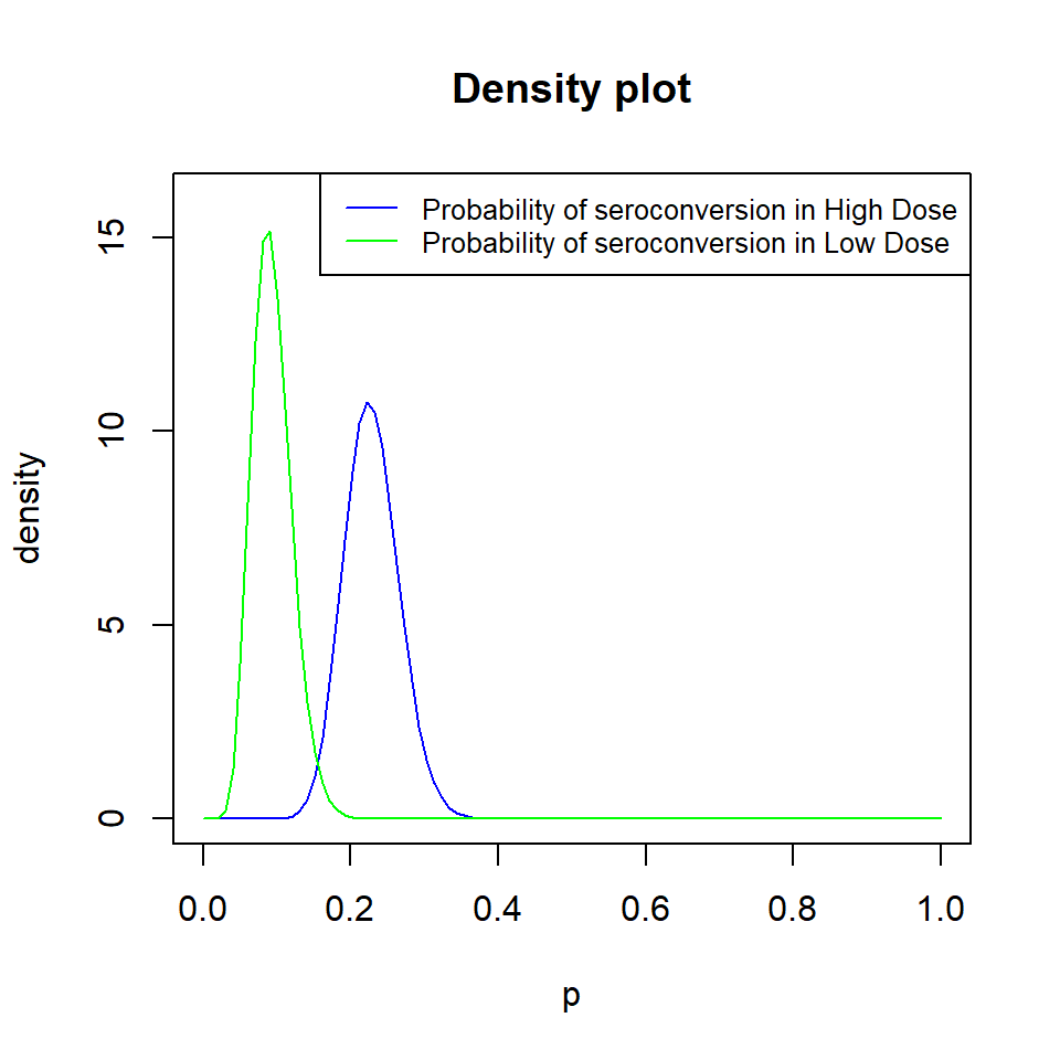
| High Dose | (0.16, 0.31) | (29.0, 98.1) |
| Low Dose | (0.049, 0.15) | (11.2, 108.0) |
Density Plot of the Two Prior Distributions
The SampleSizeProportions Library
Install and Load the library
#install.packages("SampleSizeProportions")
library(SampleSizeProportions)-
This library includes many different sample size criteria including:
- Frequentist Approach: Relies on point estimates from the previous study.
- Full Bayesian (FB) Approach: Information from previous study used for both sample size calculations and analysis.
- Mixed Bayesian/Likelihood(MBL) Approach : Information from previous study used for sample size calculation only and not analysis.
- We will now illustrate the implementation of some of these criteria.
Frequentist Sample Size Calculation
- Assume the best estimates for the unknown binomial proportions are p1.estimate and p2.estimate respectively.
- The function propdiff.freq returns the required sample sizes to attain the desired length len and confidence level level for the confidence interval for the difference between the two unknown proportions from a frequentist point of view, using a normal approximation.
propdiff.freq(len=0.1,p1.estimate = 0.225,p2.estimate = 0.0882)[1] 392- The returned value is the sample size in each of the two groups to be compared.
Full Bayesian Average Length Criterion
- Assume that prior information is available on the two proportions that can be expressed in the form Beta(c1, d1) and Beta(c2, d2) densities, respectively.
- Sample size calculation using the Full Bayesian Average Length Criterion (ALC) can be implemented as follows
propdiff.alc(c1=beta.prior.HDIIV$a, d1=beta.prior.HDIIV$b,
             c2=beta.prior.SDIIV$a, d2=beta.prior.SDIIV$b,
             len=0.1, equal = FALSE, m = 50000, mcs = 3)
[1] 327 197- The returned values are the sample sizes needed to achieve an average a posterior credible interval length of 0.1 across 50000 possible datasets while the coverage probability is fixed at 95%.
- Function arguments will be defined in greater detail on the next slide.
Arguments for propdiff.alc
- len: the desired average length of the posterior credible interval for the difference between the two unknown proportions.
- (c1, d1) and (c2, d2): the prior Beta parameters for two proportions.
- m: the number of points simulated from the preposterior distribution of the data.
- equal: boolean argument that specifies whether the final group sizes (n1, n2) are forced to be equal.
- level: the fixed coverage probability of the posterior credible interval. Default value is 0.95.
- mcs: The Maximum number of Consecutive Steps allowed in the same direction in the march towards the optimal sample size (suggested value =3).
Difference between Full Bayesian Criteria and Mixed Bayesian-Likelihood Criteria
Let \(\theta\) denote the parameter under study and \(f(\theta)\) the prior distribution of \(\theta\). Let \(x=(x_1,...,x_n)\in \mathcal{X}\) denote the data to be observed in the new study, where \(n\) is the sample size. The pre-posterior marginal distribution of the data, is:
\[ \begin{equation} f(x)=\int_\Theta f(x|\theta)f(\theta)d\theta~~~~~~~~~~~~~~~~(1) \end{equation} \] and the posterior distribution of \(\theta\) given x is: \[ \begin{equation} f(\theta|x)=\frac{f(x|\theta)f(\theta)}{\int_\Theta f(x|\theta)f(\theta)d\theta}~~~~~~~~~~~~(2) \end{equation} \] In the Fully Bayesian approach, \(f(\theta)\) is an informative prior distribution in both (1) and (2). In the Mixed Bayesian-Likelihood approach \(f(\theta)\) is informative in (1) but non-informative, e.g. uniform, in (2).
Mixed Bayesian-Likelihood Average Length Criterion
- Sample size calculation using the Full Bayesian Average Length Criterion (ALC) can be implemented as follows
Example
propdiff.mblalc(c1=beta.prior.HDIIV$a, d1=beta.prior.HDIIV$b,
                c2=beta.prior.SDIIV$a, d2=beta.prior.SDIIV$b,
                len=0.1, m = 50000, mcs = 3)
[1] 396 396- Notice that the sample size calcuated is the same in both groups because the non-informative prior distribution used at the analysis stage is the same for both groups.
Arguments for propdiff.mblalc
- len: the desired average length of the posterior credible interval for the difference between the two unknown proportions.
- (c1, d1) and (c2, d2): the pairs of prior Beta parameters for two proportions.
- m: the number of points simulated from the preposterior distribution of the data.
- level: the fixed coverage probability of the posterior credible interval. Default value is 0.95.
- mcs: The Maximum number of Consecutive Steps allowed in the same direction in the march towards the optimal sample size (suggested value =3).
Other Bayesian Criteria in the Library
- Besides the two average length criteria illustrated, a number of other criteria are available:
- Full Bayesian (FB):
- the Average Coverage Criterion (ACC): propdiff.acc.
- the Worst Outcome Criterion (WOC): propdiff.woc.
- the Modified Worst Outcome Criterion (mWOC): propdiff.modwoc.
- Mixed Bayesian Likelihood (MBL):
- the Mixed Bayesian/Likelihood Average Coverage Criterion (MBLACC): propdiff.mblacc.
- the Mixed Bayesian/Likelihood Worst Outcome Criterion (MBLWOC): propdiff.mblwoc.
- the Mixed Bayesian/Likelihood Modified Worst Outcome Criterion (MBLMODWOC): propdiff.mblmodwoc.
- Full Bayesian (FB):
Table 1: Comparing different criteria when len=0.1, level=0.95
- The table below gives the results of applying different criteria to our motivating example:
| Criterion | High.Dose | Low.Dose |
|---|---|---|
| Frequentist | 392 | 392 |
| Bayesian, ALC, non-informative prior | 392 | 392 |
| Bayesian, ACC, non-informative prior | 394 | 394 |
| Bayesian, mWOC (0.95), non-informative prior | 510 | 510 |
| Bayesian, ALC, informative prior | 323 | 192 |
| Bayesian, ACC, informative prior | 325 | 194 |
| Bayesian, mWOC (0.95), informative prior | 361 | 371 |
Discussion of Table 1
In the results, you may notice that
- The mWOC (0.95) criterion yields larger values of the sample size needed than ALC or ACC does.
- This is because that the mWOC (0.95) is a more conservative criterion that ensure the desired length and coverage are obtained in 95% of possible datasets while the ACC and ALC criteria are based on averages across possible datasets.
- Smaller sample sizes are needed when informative priors are used (red) compared to non-informative priors or the frequentist approach(blue).
- Further, as Joseph, Berger, and Belisle (1997) discussed, the Fully Bayesian criteria result in sample sizes that are uniformly smaller than the Mixed Bayesian-Likelihood criteria.
- The availability of prior information also permits us to collect less information on one of the proportions if its prior is more informative. However, the sample sizes can be forced to be equal if that is more convenient for practical reasons
Table 2: Comparing different criteria when len=0.2, level=0.95
- The table below gives the results of applying the different criteria to the same example but with the desired interval length set to be wider:
| Criterion | High.Dose | Low.Dose |
|---|---|---|
| Frequentist | 98 | 98 |
| Bayesian, ALC, non-informative prior | 98 | 98 |
| Bayesian, ACC, non-informative prior | 99 | 99 |
| Bayesian, mWOC (0.95), non-informative prior | 134 | 134 |
| Bayesian, ALC, informative prior | 0 | 0 |
| Bayesian, ACC, informative prior | 0 | 0 |
| Bayesian, mWOC (0.95), informative prior | 0 | 0 |
Discussion of Table 2
In the results, you may notice that
- Both Full Bayesian and Mixed Bayesian-Likelihood criteria result in dramatically smaller sample sizes.
- The sample sizes needed can even reduce to 0 if the prior information is sufficiently informative and no additional data are necessary to achieve the desired precision (or interval length).
- Thank you! Please send any questions or comments to nandini.dendukuri@mcgill.ca.
References
Joseph, Lawrence, Roxane Du Berger, and Patrick Belisle. 1997. “Bayesian and Mixed Bayesian/Likelihood Criteria for Sample Size Determination.” Statistics in Medicine 16 (7): 769–81. https://doi.org/10.1002/(sici)1097-0258(19970415)16:7<769::aid-sim495>3.0.co;2-v.
Press, S. James. 1989. Bayesian Statistics Principles, Models and Applications. John Wiley & Sons.
Citation
BibTeX citation:
@online{lu2019,
  author = {Yang Lu and Nandini Dendukuri},
  title = {Bayesian {Sample} {Size} {Calculations} for {Difference} in
    {Proportions}},
  date = {2019-09-19},
  url = {https://www.nandinidendukuri.com/blogposts/2019-09-19-bayes-sampsize-difference-proportions/},
  langid = {en}
}
For attribution, please cite this work as:
Yang Lu, and Nandini Dendukuri. 2019. “Bayesian Sample Size
Calculations for Difference in Proportions.” September 19, 2019.
https://www.nandinidendukuri.com/blogposts/2019-09-19-bayes-sampsize-difference-proportions/.